
Color-magnitude diagram: broadband filters
This tutorial shows how to create a color-magnitude diagram that includes data of field and young/low-gravity objects, synthetic photometry computed from isochrones and model spectra, and data of directly imaged objects.
Initiating species
We start by importing the required modules.
[1]:
import numpy as np
from species import SpeciesInit
from species.data.database import Database
from species.read.read_color import ReadColorMagnitude
from species.read.read_isochrone import ReadIsochrone
from species.read.read_planck import ReadPlanck
from species.plot.plot_spectrum import plot_spectrum
from species.plot.plot_color import plot_color_magnitude
WARNING: AstropyDeprecationWarning: astropy.samp was deprecated in version 8.0 and will be removed in a future version; please use pyvo.samp instead. [astropy.samp]
Next, we initiate the species workflow and create an instance of Database.
[2]:
SpeciesInit()
database = Database()
=======
species
=======

Version: 0.10.5.dev13
Working folder: /Users/tomasstolker/code/species/docs/tutorials

Creating species_config.ini... [DONE]
Creating species_database.hdf5... [DONE]
Creating data folder... [DONE]

Configuration settings:
   - Database: species_database.hdf5
   - Data folder: data
   - Magnitude of Vega: 0.03

Multiprocessing: mpi4py installed
Process number 1 out of 1...
Adding data to the database
Available magnitudes and spectra of directly imaged planets and brown dwarfs are added to the database with add_companion by setting name=None. These data are extracted from the companion_data and
companion_spectra files in the companion_data subpackage.
[3]:
database.add_companion(name=None, verbose=False)
Add companion: ['HD 135344 Ab', 'AF Lep b', 'beta Pic b', 'beta Pic c', 'beta Pic d', 'HIP 65426 b', 'HIP 99770 b', '51 Eri b', 'HR 8799 b', 'HR 8799 c', 'HR 8799 d', 'HR 8799 e', 'HD 95086 b', 'PDS 70 b', 'PDS 70 c', '2M 1207 B', 'AB Pic B', 'HD 206893 B', 'HD 206893 c', 'RZ Psc B', 'GQ Lup B', 'PZ Tel B', 'kappa And b', 'HD 1160 B', 'ROXs 12 B', 'ROXs 42 Bb', 'GJ 504 b', 'GJ 758 B', 'GU Psc b', '2M0103 ABb', '1RXS 1609 B', 'GSC 06214 B', 'HD 72946 B', 'HIP 64892 B', 'HD 13724 B', 'YSES 1 b', 'YSES 1 c', 'HD 142527 B', 'CS Cha B', 'CT Cha B', 'SR 12 C', 'DH Tau B', 'HD 4747 B', 'HR 3549 B', 'CHXR 73 B', 'HD 19467 B', 'b Cen (AB)b', 'eps Ind Ab', 'WISPIT 2 b', 'VHS 1256 B']
Downloading data from 'https://archive.stsci.edu/hlsps/reference-atlases/cdbs/current_calspec/alpha_lyr_stis_011.fits' to file '/Users/tomasstolker/code/species/docs/tutorials/data/alpha_lyr_stis_011.fits'.
Downloading data from 'https://home.strw.leidenuniv.nl/~stolker/species/alpha_lyr_stis_011.fits' to file '/Users/tomasstolker/code/species/docs/tutorials/data/alpha_lyr_stis_011.fits'.
Adding spectrum: Vega
Downloading data from 'https://home.strw.leidenuniv.nl/~stolker/species/spectra/betapicb_gpi_yjhk.dat' to file '/Users/tomasstolker/code/species/docs/tutorials/data/companion_data/betapicb_gpi_yjhk.dat'.
Reference: Bohlin et al. 2014, PASP, 126
URL: https://ui.adsabs.harvard.edu/abs/2014PASP..126..711B
SHA256 hash of downloaded file: 33e8d3ee32aa661f97624eda64e4a7f67dac2a7f22a072136a8414713379ef50
Use this value as the 'known_hash' argument of 'pooch.retrieve' to ensure that the file hasn't changed if it is downloaded again in the future.
Downloading data from 'https://home.strw.leidenuniv.nl/~stolker/species/spectra/BetaPictorisb_2018-09-22.fits' to file '/Users/tomasstolker/code/species/docs/tutorials/data/companion_data/BetaPictorisb_2018-09-22.fits'.
SHA256 hash of downloaded file: 4b4507e4af6cec5711d2110974061584b8d23cc108daae7fa3be8c27d866847c
Use this value as the 'known_hash' argument of 'pooch.retrieve' to ensure that the file hasn't changed if it is downloaded again in the future.
Downloading data from 'https://xwcl.science/magao/visao/VisAO_Ys_filter_curve.dat' to file '/Users/tomasstolker/code/species/docs/tutorials/data/VisAO_Ys_filter_curve.dat'.
SHA256 hash of downloaded file: 4d523a06d8daae91f91d98f4ee8dacbfef7d17c6161a4c217dd56cd6006b9d56
Use this value as the 'known_hash' argument of 'pooch.retrieve' to ensure that the file hasn't changed if it is downloaded again in the future.
/Users/tomasstolker/code/species/species/data/database.py:1535: UserWarning: Found 33 fluxes with NaN in the data of GPI_YJHK. Removing the spectral fluxes that contain a NaN.
  warnings.warn(
Downloading data from 'https://home.strw.leidenuniv.nl/~stolker/species/spectra/51erib_sphere_yjh.dat' to file '/Users/tomasstolker/code/species/docs/tutorials/data/companion_data/51erib_sphere_yjh.dat'.
SHA256 hash of downloaded file: d050f0a5762b2fb277284fd7a514c9656605d720ee4dab1b61c35f05256d16a9
Use this value as the 'known_hash' argument of 'pooch.retrieve' to ensure that the file hasn't changed if it is downloaded again in the future.
/Users/tomasstolker/code/species/species/data/filter_data/filter_data.py:374: UserWarning: The minimum transmission value of Subaru/CIAO.z is smaller than zero (-1.80e-03). Wavelengths with negative transmission values will be removed.
  warnings.warn(
Downloading data from 'https://home.strw.leidenuniv.nl/~stolker/species/spectra/hr8799e_sphere_yjh.dat' to file '/Users/tomasstolker/code/species/docs/tutorials/data/companion_data/hr8799e_sphere_yjh.dat'.
SHA256 hash of downloaded file: 8807ff91d417513b6f4ca2c5a21e68830830c81cd8ef7399260de8796d72496b
Use this value as the 'known_hash' argument of 'pooch.retrieve' to ensure that the file hasn't changed if it is downloaded again in the future.
Downloading data from 'https://home.strw.leidenuniv.nl/~stolker/species/spectra/pds70b_sphere_yjh.dat' to file '/Users/tomasstolker/code/species/docs/tutorials/data/companion_data/pds70b_sphere_yjh.dat'.
SHA256 hash of downloaded file: d9ca1a0e4783bed66ab8512a5939927d3846bf82ac16981565747f2e9459fc0b
Use this value as the 'known_hash' argument of 'pooch.retrieve' to ensure that the file hasn't changed if it is downloaded again in the future.
Downloading data from 'https://home.strw.leidenuniv.nl/~stolker/species/spectra/hd206893b_sphere_yjh.dat' to file '/Users/tomasstolker/code/species/docs/tutorials/data/companion_data/hd206893b_sphere_yjh.dat'.
SHA256 hash of downloaded file: 676f9140257b0e5fd70a6ae8c95e8543d59a83b16dd4cab0ddcb0dcc41544f35
Use this value as the 'known_hash' argument of 'pooch.retrieve' to ensure that the file hasn't changed if it is downloaded again in the future.
Downloading data from 'https://home.strw.leidenuniv.nl/~stolker/species/spectra/HD206893C_GRAVITYK_fluxcal_spectrum.fits' to file '/Users/tomasstolker/code/species/docs/tutorials/data/companion_data/HD206893C_GRAVITYK_fluxcal_spectrum.fits'.
SHA256 hash of downloaded file: abacbf0435af6f5b06ff4f01567dbdc37e529e9f7ba5ddfc588ce73a4df0b43b
Use this value as the 'known_hash' argument of 'pooch.retrieve' to ensure that the file hasn't changed if it is downloaded again in the future.
Downloading data from 'https://home.strw.leidenuniv.nl/~stolker/species/spectra/gqlupb_muse.dat' to file '/Users/tomasstolker/code/species/docs/tutorials/data/companion_data/gqlupb_muse.dat'.
SHA256 hash of downloaded file: a96bb9e2de04cd001cd5cf1c5297eaed88eb0a888bc41e6b2d861c8d47e9db56
Use this value as the 'known_hash' argument of 'pooch.retrieve' to ensure that the file hasn't changed if it is downloaded again in the future.
Downloading data from 'https://home.strw.leidenuniv.nl/~stolker/species/spectra/gqlupb_sinfoni_j.dat' to file '/Users/tomasstolker/code/species/docs/tutorials/data/companion_data/gqlupb_sinfoni_j.dat'.
SHA256 hash of downloaded file: 8667316e76424eb64a8816cbec7e1359a502304bcafcc6fb326af840ecec0eed
Use this value as the 'known_hash' argument of 'pooch.retrieve' to ensure that the file hasn't changed if it is downloaded again in the future.
Downloading data from 'https://home.strw.leidenuniv.nl/~stolker/species/spectra/gqlupb_sinfoni_h.dat' to file '/Users/tomasstolker/code/species/docs/tutorials/data/companion_data/gqlupb_sinfoni_h.dat'.
SHA256 hash of downloaded file: 1a8b0ecb0908076d0a347fe5d0b0ae7a615daaf0be525c7a642fe57d003e9566
Use this value as the 'known_hash' argument of 'pooch.retrieve' to ensure that the file hasn't changed if it is downloaded again in the future.
Downloading data from 'https://home.strw.leidenuniv.nl/~stolker/species/spectra/gqlupb_sinfoni_k.dat' to file '/Users/tomasstolker/code/species/docs/tutorials/data/companion_data/gqlupb_sinfoni_k.dat'.
SHA256 hash of downloaded file: d2e62c8f9e803cc06d6d3b85a78c23b202e0742b97e8e27a717cf251ba5513bf
Use this value as the 'known_hash' argument of 'pooch.retrieve' to ensure that the file hasn't changed if it is downloaded again in the future.
Downloading data from 'https://xwcl.science/magao/visao/VisAO_ip_filter_curve.dat' to file '/Users/tomasstolker/code/species/docs/tutorials/data/VisAO_ip_filter_curve.dat'.
SHA256 hash of downloaded file: cbda362353fe25b78bec67506288fa6220ca22228cb7ddf94d5fcf8bc2a4dfb3
Use this value as the 'known_hash' argument of 'pooch.retrieve' to ensure that the file hasn't changed if it is downloaded again in the future.
Downloading data from 'https://xwcl.science/magao/visao/VisAO_zp_filter_curve.dat' to file '/Users/tomasstolker/code/species/docs/tutorials/data/VisAO_zp_filter_curve.dat'.
SHA256 hash of downloaded file: 8d1ee51d7e52beb2fd1d6405c2bc1b83f2691324c2dba609b4f97de4b30329bd
Use this value as the 'known_hash' argument of 'pooch.retrieve' to ensure that the file hasn't changed if it is downloaded again in the future.
Downloading data from 'https://home.strw.leidenuniv.nl/~stolker/species/filters/Keck_NIRC2.NB_4.05.dat' to file '/Users/tomasstolker/code/species/docs/tutorials/data/Keck_NIRC2.NB_4.05.dat'.
We also add the photometry and parallaxes of the Database of Ultracool Parallaxes.
[4]:
database.add_photometry('vlm-plx')
Downloading data from 'https://home.strw.leidenuniv.nl/~stolker/species/vlm-plx-all.fits' to file '/Users/tomasstolker/code/species/docs/tutorials/data/vlm-plx-all.fits'.
-----------------------
Add photometric library
-----------------------

Database tag: vlm-plx
Library: Database of Ultracool Parallaxes
Next, we add the isochrones from AMES-Cond and AMES-Dusty, which have been retrieved from https://phoenix.ens-lyon.fr/Grids/.
[5]:
database.add_isochrones('ames')
Downloading data from 'https://home.strw.leidenuniv.nl/~stolker/species/model.AMES-Cond-2000.M-0.0.MKO.Vega' to file '/Users/tomasstolker/code/species/docs/tutorials/data/model.AMES-Cond-2000.M-0.0.MKO.Vega'.
------------------
Add isochrone grid
------------------

Evolutionary model: ames
File name: None
Database tag: None
Adding isochrones: ames-cond...
Downloading data from 'https://home.strw.leidenuniv.nl/~stolker/species/model.AMES-dusty.M-0.0.MKO.Vega' to file '/Users/tomasstolker/code/species/docs/tutorials/data/model.AMES-dusty.M-0.0.MKO.Vega'.
 [DONE]
Database tag: ames-cond
Adding isochrones: ames-dusty... [DONE]
Database tag: ames-dusty
Finally, we need to add the grid with AMES-Cond model spectra. The full grid of spectra is downloaded but spectra with a \(T_\mathrm{eff}\) outside the chosen teff_range are not added to the database.
[6]:
database.add_model(model='ames-cond',
                   teff_range=(100., 4000.))
Downloading data from 'https://home.strw.leidenuniv.nl/~stolker/species/ames-cond.tgz' to file '/Users/tomasstolker/code/species/docs/tutorials/data/ames-cond.tgz'.
-------------------------
Add grid of model spectra
-------------------------

Database tag: ames-cond
Model name: AMES-Cond
Unpacking 278/439 model spectra from AMES-Cond (57 MB)... [DONE]

Please cite Allard et al. (2001) when using AMES-Cond in a publication
Reference URL: https://ui.adsabs.harvard.edu/abs/2001ApJ...556..357A

Wavelength range (um) = 0.5 - 40
Sampling (lambda/d_lambda) = 2000
Teff range (K) = 100.0 - 4000.0

Adding AMES-Cond model spectra... data/ames-cond/ames-cond_teff_900_logg_5.5_spec.npy

Grid points stored in the database:
   - Teff = [ 100.  200.  300.  400.  500.  600.  700.  800.  900. 1000. 1100. 1200.
 1300. 1400. 1500. 1600. 1700. 1800. 1900. 2000. 2100. 2200. 2300. 2400.
 2500. 2600. 2700. 2800. 2900. 3000. 3100. 3200. 3300. 3400. 3500. 3600.
 3700. 3800. 3900. 4000.]
   - log(g) = [2.5 3.  3.5 4.  4.5 5.  5.5]

Number of grid points per parameter:
   - teff: 40
   - logg: 7

Fix missing grid points with a linear interpolation:
   - teff = 200.0, logg = 5.5
   - teff = 900.0, logg = 2.5

Number of stored grid points: 280
Number of interpolated grid points: 2
Number of missing grid points: 0
/Users/tomasstolker/code/species/species/util/data_util.py:414: RuntimeWarning: divide by zero encountered in log10
  flux = np.log10(flux)
Also the AMES-Dusty spectra are downloaded and imported into the database.
[7]:
database.add_model(model='ames-dusty',
                   teff_range=(100., 4000.))
Downloading data from 'https://home.strw.leidenuniv.nl/~stolker/species/ames-dusty.tgz' to file '/Users/tomasstolker/code/species/docs/tutorials/data/ames-dusty.tgz'.
-------------------------
Add grid of model spectra
-------------------------

Database tag: ames-dusty
Model name: AMES-Dusty
Unpacking 195/195 model spectra from AMES-Dusty (22 MB)... [DONE]

Please cite Allard et al. (2001) when using AMES-Dusty in a publication
Reference URL: https://ui.adsabs.harvard.edu/abs/2001ApJ...556..357A

Wavelength range (um) = 0.5 - 40
Sampling (lambda/d_lambda) = 2000
Teff range (K) = 100.0 - 4000.0

Adding AMES-Dusty model spectra... data/ames-dusty/ames-dusty_teff_900_logg_5.5_spec.npy

Grid points stored in the database:
   - Teff = [ 500.  600.  700.  800.  900. 1000. 1100. 1200. 1300. 1400. 1500. 1600.
 1700. 1800. 1900. 2000. 2100. 2200. 2300. 2400. 2500. 2600. 2700. 2800.
 2900. 3000. 3100. 3200. 3300. 3400. 3500. 3600. 3700. 3800. 3900. 4000.]
   - log(g) = [3.5 4.  4.5 5.  5.5 6. ]

Number of grid points per parameter:
   - teff: 36
   - logg: 6

Fix missing grid points with a linear interpolation:
   - teff = 900.0, logg = 6.0
   - teff = 1200.0, logg = 5.5
   - teff = 2100.0, logg = 3.5
   - teff = 2100.0, logg = 4.5
   - teff = 2200.0, logg = 3.5
   - teff = 2400.0, logg = 5.0
   - teff = 3100.0, logg = 3.5
   - teff = 3200.0, logg = 3.5
   - teff = 3300.0, logg = 3.5
   - teff = 3400.0, logg = 3.5
   - teff = 3500.0, logg = 3.5
   - teff = 3600.0, logg = 3.5
   - teff = 3700.0, logg = 3.5
   - teff = 3800.0, logg = 3.5
   - teff = 3900.0, logg = 3.5
   - teff = 3900.0, logg = 6.0
   - teff = 4000.0, logg = 3.5
   - teff = 4000.0, logg = 4.0
   - teff = 4000.0, logg = 4.5
   - teff = 4000.0, logg = 5.5
   - teff = 4000.0, logg = 6.0

The following grid points are missing:
   - teff = 3100.0, logg = 3.5
   - teff = 3200.0, logg = 3.5
   - teff = 3300.0, logg = 3.5
   - teff = 3400.0, logg = 3.5
   - teff = 3500.0, logg = 3.5
   - teff = 3600.0, logg = 3.5
   - teff = 3700.0, logg = 3.5
   - teff = 3800.0, logg = 3.5
   - teff = 3900.0, logg = 3.5
   - teff = 3900.0, logg = 6.0
   - teff = 4000.0, logg = 3.5
   - teff = 4000.0, logg = 4.0
   - teff = 4000.0, logg = 4.5
   - teff = 4000.0, logg = 5.5
   - teff = 4000.0, logg = 6.0

Number of stored grid points: 216
Number of interpolated grid points: 6
Number of missing grid points: 15
/Users/tomasstolker/code/species/species/util/data_util.py:414: RuntimeWarning: divide by zero encountered in log10
  flux = np.log10(flux)
/Users/tomasstolker/code/species/species/util/data_util.py:498: UserWarning: Could not interpolate 15 grid points so storing zeros instead.
  warnings.warn(
We are now ready with preparing the HDF5 database. The list_content method of the Database object can be used for printing an overview of all the data that are stored in the database.
Synthetic photometry from isochrones
Magnitudes from the isochrone data can be extracted with the get_isochrone function of ReadIsochrone. However, in this example, we consistently recompute the synthetic photometry by making use of both the evolutionary tracks and the synthetic spectra.
The isochrones will be iterpolated for three different ages and the synthetic photometry is computed at 100 logarithmically-spaced masses.
[8]:
ages = [20., 100.]  # (Myr)
masses = np.logspace(0., 3., 100)  # (Mjup)
We create instances of ReadIsochrone for both the AMES-Cond and AMES-Dusty isochrones. We note though that the evolutionary data of these two models are actually the same. Only the magnitudes of the isochrones (which we do not use) are different.
[9]:
read_iso_cond = ReadIsochrone(tag='ames-cond')
read_iso_dusty = ReadIsochrone(tag='ames-dusty')
-------------------
Read isochrone grid
-------------------

Database tag: ames-cond
Create regular grid: False

Setting 'extra_param' attribute: None

-------------------
Read isochrone grid
-------------------

Database tag: ames-dusty
Create regular grid: False

Setting 'extra_param' attribute: None
The colors and magnitudes are computed by chosing the corresponding model grids from the database. The output is stored in ColorMagBox objects for the three different ages.
[10]:
boxes = []

for item in ages:

    modelcolor1 = read_iso_cond.get_color_magnitude(age=item,
                                                    masses=masses,
                                                    filters_color=('MKO/NSFCam.H', 'MKO/NSFCam.Lp'),
                                                    filter_mag='MKO/NSFCam.Lp')

    modelcolor2 = read_iso_dusty.get_color_magnitude(age=item,
                                                     masses=masses,
                                                     filters_color=('MKO/NSFCam.H', 'MKO/NSFCam.Lp'),
                                                     filter_mag='MKO/NSFCam.Lp')

    boxes.append(modelcolor1)
    boxes.append(modelcolor2)
/Users/tomasstolker/code/species/species/read/read_isochrone.py:1407: UserWarning: The value of teff is 4019.3207105807364, which is above the upper bound of the model grid (4000.0). Setting the magnitudes to NaN for the following isochrone sample: {'teff': np.float64(4019.3207105807364), 'logg': np.float64(4.351948444496957), 'radius': np.float64(10.170788710818774), 'distance': 10.0}.
  warnings.warn(
/Users/tomasstolker/code/species/species/read/read_isochrone.py:1407: UserWarning: The value of teff is 4164.404431717177, which is above the upper bound of the model grid (4000.0). Setting the magnitudes to NaN for the following isochrone sample: {'teff': np.float64(4164.404431717177), 'logg': np.float64(4.329081153206135), 'radius': np.float64(10.739016824226589), 'distance': 10.0}.
  warnings.warn(
/Users/tomasstolker/code/species/species/read/read_isochrone.py:1382: UserWarning: The value of logg is 2.9180307893338333, which is below the lower bound of the model grid (3.5). Setting the magnitudes to NaN for the following isochrone sample: {'teff': np.float64(501.3730414241426), 'logg': np.float64(2.9180307893338333), 'radius': np.float64(1.4638670830301985), 'distance': 10.0}.
  warnings.warn(
/Users/tomasstolker/code/species/species/read/read_isochrone.py:1382: UserWarning: The value of logg is 2.9730768802029495, which is below the lower bound of the model grid (3.5). Setting the magnitudes to NaN for the following isochrone sample: {'teff': np.float64(502.52702926884206), 'logg': np.float64(2.9730768802029495), 'radius': np.float64(1.4416707276599539), 'distance': 10.0}.
  warnings.warn(
/Users/tomasstolker/code/species/species/read/read_isochrone.py:1382: UserWarning: The value of logg is 3.035563154856569, which is below the lower bound of the model grid (3.5). Setting the magnitudes to NaN for the following isochrone sample: {'teff': np.float64(504.9233097703563), 'logg': np.float64(3.035563154856569), 'radius': np.float64(1.415090361603327), 'distance': 10.0}.
  warnings.warn(
/Users/tomasstolker/code/species/species/read/read_isochrone.py:1382: UserWarning: The value of logg is 3.1025651389931808, which is below the lower bound of the model grid (3.5). Setting the magnitudes to NaN for the following isochrone sample: {'teff': np.float64(507.49276280687246), 'logg': np.float64(3.1025651389931808), 'radius': np.float64(1.3865891063317703), 'distance': 10.0}.
  warnings.warn(
/Users/tomasstolker/code/species/species/read/read_isochrone.py:1382: UserWarning: The value of logg is 3.207337823869265, which is below the lower bound of the model grid (3.5). Setting the magnitudes to NaN for the following isochrone sample: {'teff': np.float64(520.0556848108937), 'logg': np.float64(3.207337823869265), 'radius': np.float64(1.328194511799377), 'distance': 10.0}.
  warnings.warn(
/Users/tomasstolker/code/species/species/read/read_isochrone.py:1382: UserWarning: The value of logg is 3.30652717870104, which is below the lower bound of the model grid (3.5). Setting the magnitudes to NaN for the following isochrone sample: {'teff': np.float64(534.0174915985032), 'logg': np.float64(3.30652717870104), 'radius': np.float64(1.274758290992437), 'distance': 10.0}.
  warnings.warn(
/Users/tomasstolker/code/species/species/read/read_isochrone.py:1382: UserWarning: The value of logg is 3.3387964574578715, which is below the lower bound of the model grid (3.5). Setting the magnitudes to NaN for the following isochrone sample: {'teff': np.float64(543.9916323051602), 'logg': np.float64(3.3387964574578715), 'radius': np.float64(1.2725698348137873), 'distance': 10.0}.
  warnings.warn(
/Users/tomasstolker/code/species/species/read/read_isochrone.py:1382: UserWarning: The value of logg is 3.372282732356024, which is below the lower bound of the model grid (3.5). Setting the magnitudes to NaN for the following isochrone sample: {'teff': np.float64(556.2475974396231), 'logg': np.float64(3.372282732356024), 'radius': np.float64(1.2706911157956755), 'distance': 10.0}.
  warnings.warn(
/Users/tomasstolker/code/species/species/read/read_isochrone.py:1382: UserWarning: The value of logg is 3.407135965646942, which is below the lower bound of the model grid (3.5). Setting the magnitudes to NaN for the following isochrone sample: {'teff': np.float64(570.8634694648467), 'logg': np.float64(3.407135965646942), 'radius': np.float64(1.269118495295348), 'distance': 10.0}.
  warnings.warn(
/Users/tomasstolker/code/species/species/read/read_isochrone.py:1382: UserWarning: The value of logg is 3.444507945285873, which is below the lower bound of the model grid (3.5). Setting the magnitudes to NaN for the following isochrone sample: {'teff': np.float64(586.5355899585919), 'logg': np.float64(3.444507945285873), 'radius': np.float64(1.2674322258801856), 'distance': 10.0}.
  warnings.warn(
/Users/tomasstolker/code/species/species/read/read_isochrone.py:1382: UserWarning: The value of logg is 3.484580694074335, which is below the lower bound of the model grid (3.5). Setting the magnitudes to NaN for the following isochrone sample: {'teff': np.float64(603.3402910634309), 'logg': np.float64(3.484580694074335), 'radius': np.float64(1.2656240944588282), 'distance': 10.0}.
  warnings.warn(
/Users/tomasstolker/code/species/species/read/read_isochrone.py:1407: UserWarning: The value of teff is 4081.435563185969, which is above the upper bound of the model grid (4000.0). Setting the magnitudes to NaN for the following isochrone sample: {'teff': np.float64(4081.435563185969), 'logg': np.float64(4.66798518435126), 'radius': np.float64(5.914180524946678), 'distance': 10.0}.
  warnings.warn(
/Users/tomasstolker/code/species/species/read/read_isochrone.py:1407: UserWarning: The value of teff is 4185.2608377397555, which is above the upper bound of the model grid (4000.0). Setting the magnitudes to NaN for the following isochrone sample: {'teff': np.float64(4185.2608377397555), 'logg': np.float64(4.656638159809863), 'radius': np.float64(6.199078262481065), 'distance': 10.0}.
  warnings.warn(
/Users/tomasstolker/code/species/species/read/read_isochrone.py:1407: UserWarning: The value of teff is 4325.615910494432, which is above the upper bound of the model grid (4000.0). Setting the magnitudes to NaN for the following isochrone sample: {'teff': np.float64(4325.615910494432), 'logg': np.float64(4.641153787722841), 'radius': np.float64(6.55382759835061), 'distance': 10.0}.
  warnings.warn(
/Users/tomasstolker/code/species/species/read/read_isochrone.py:1407: UserWarning: The value of teff is 4512.024881795706, which is above the upper bound of the model grid (4000.0). Setting the magnitudes to NaN for the following isochrone sample: {'teff': np.float64(4512.024881795706), 'logg': np.float64(4.610559348746732), 'radius': np.float64(7.038423776652953), 'distance': 10.0}.
  warnings.warn(
/Users/tomasstolker/code/species/species/read/read_isochrone.py:1407: UserWarning: The value of teff is 4704.664806542345, which is above the upper bound of the model grid (4000.0). Setting the magnitudes to NaN for the following isochrone sample: {'teff': np.float64(4704.664806542345), 'logg': np.float64(4.571845570260295), 'radius': np.float64(7.623463332054268), 'distance': 10.0}.
  warnings.warn(
/Users/tomasstolker/code/species/species/read/read_isochrone.py:1407: UserWarning: The value of teff is 4915.122843504474, which is above the upper bound of the model grid (4000.0). Setting the magnitudes to NaN for the following isochrone sample: {'teff': np.float64(4915.122843504474), 'logg': np.float64(4.527793777987827), 'radius': np.float64(8.265784389535268), 'distance': 10.0}.
  warnings.warn(
/Users/tomasstolker/code/species/species/read/read_isochrone.py:1407: UserWarning: The value of teff is 5129.690817228589, which is above the upper bound of the model grid (4000.0). Setting the magnitudes to NaN for the following isochrone sample: {'teff': np.float64(5129.690817228589), 'logg': np.float64(4.487243459618406), 'radius': np.float64(8.971175402210688), 'distance': 10.0}.
  warnings.warn(
/Users/tomasstolker/code/species/species/read/read_isochrone.py:1382: UserWarning: The value of logg is 2.796196997524488, which is below the lower bound of the model grid (3.5). Setting the magnitudes to NaN for the following isochrone sample: {'teff': np.float64(501.5843871005805), 'logg': np.float64(2.796196997524488), 'radius': np.float64(1.5064919873572373), 'distance': 10.0}.
  warnings.warn(
/Users/tomasstolker/code/species/species/read/read_isochrone.py:1382: UserWarning: The value of logg is 2.8072667505973876, which is below the lower bound of the model grid (3.5). Setting the magnitudes to NaN for the following isochrone sample: {'teff': np.float64(501.6880174178661), 'logg': np.float64(2.8072667505973876), 'radius': np.float64(1.5031419477567407), 'distance': 10.0}.
  warnings.warn(
/Users/tomasstolker/code/species/species/read/read_isochrone.py:1382: UserWarning: The value of logg is 2.820805889271204, which is below the lower bound of the model grid (3.5). Setting the magnitudes to NaN for the following isochrone sample: {'teff': np.float64(501.6648632173275), 'logg': np.float64(2.820805889271204), 'radius': np.float64(1.4989194659748202), 'distance': 10.0}.
  warnings.warn(
/Users/tomasstolker/code/species/species/read/read_isochrone.py:1382: UserWarning: The value of logg is 2.835323463885389, which is below the lower bound of the model grid (3.5). Setting the magnitudes to NaN for the following isochrone sample: {'teff': np.float64(501.640035727038), 'logg': np.float64(2.835323463885389), 'radius': np.float64(1.4943918371645313), 'distance': 10.0}.
  warnings.warn(
/Users/tomasstolker/code/species/species/read/read_isochrone.py:1382: UserWarning: The value of logg is 2.8556700278606737, which is below the lower bound of the model grid (3.5). Setting the magnitudes to NaN for the following isochrone sample: {'teff': np.float64(501.65383479103104), 'logg': np.float64(2.8556700278606737), 'radius': np.float64(1.4883035183626285), 'distance': 10.0}.
  warnings.warn(
/Users/tomasstolker/code/species/species/read/read_isochrone.py:1382: UserWarning: The value of logg is 2.8799279682862924, which is below the lower bound of the model grid (3.5). Setting the magnitudes to NaN for the following isochrone sample: {'teff': np.float64(501.6892732862044), 'logg': np.float64(2.8799279682862924), 'radius': np.float64(1.4811452905054687), 'distance': 10.0}.
  warnings.warn(
/Users/tomasstolker/code/species/species/read/read_isochrone.py:1382: UserWarning: The value of logg is 2.9059389626781624, which is below the lower bound of the model grid (3.5). Setting the magnitudes to NaN for the following isochrone sample: {'teff': np.float64(501.7272728229761), 'logg': np.float64(2.9059389626781624), 'radius': np.float64(1.4734697574065547), 'distance': 10.0}.
  warnings.warn(
/Users/tomasstolker/code/species/species/read/read_isochrone.py:1382: UserWarning: The value of logg is 2.9339822921321925, which is below the lower bound of the model grid (3.5). Setting the magnitudes to NaN for the following isochrone sample: {'teff': np.float64(501.84752531806237), 'logg': np.float64(2.9339822921321925), 'radius': np.float64(1.465193882836573), 'distance': 10.0}.
  warnings.warn(
/Users/tomasstolker/code/species/species/read/read_isochrone.py:1382: UserWarning: The value of logg is 2.9644919021316207, which is below the lower bound of the model grid (3.5). Setting the magnitudes to NaN for the following isochrone sample: {'teff': np.float64(502.20555197078556), 'logg': np.float64(2.9644919021316207), 'radius': np.float64(1.4561883961908295), 'distance': 10.0}.
  warnings.warn(
/Users/tomasstolker/code/species/species/read/read_isochrone.py:1382: UserWarning: The value of logg is 3.0026726111414517, which is below the lower bound of the model grid (3.5). Setting the magnitudes to NaN for the following isochrone sample: {'teff': np.float64(503.0100115950047), 'logg': np.float64(3.0026726111414517), 'radius': np.float64(1.444958697353407), 'distance': 10.0}.
  warnings.warn(
/Users/tomasstolker/code/species/species/read/read_isochrone.py:1382: UserWarning: The value of logg is 3.0444294083637637, which is below the lower bound of the model grid (3.5). Setting the magnitudes to NaN for the following isochrone sample: {'teff': np.float64(503.9354554753856), 'logg': np.float64(3.0444294083637637), 'radius': np.float64(1.4326823296312547), 'distance': 10.0}.
  warnings.warn(
/Users/tomasstolker/code/species/species/read/read_isochrone.py:1382: UserWarning: The value of logg is 3.0892038533213797, which is below the lower bound of the model grid (3.5). Setting the magnitudes to NaN for the following isochrone sample: {'teff': np.float64(504.92777861412816), 'logg': np.float64(3.0892038533213797), 'radius': np.float64(1.4195187829174452), 'distance': 10.0}.
  warnings.warn(
/Users/tomasstolker/code/species/species/read/read_isochrone.py:1382: UserWarning: The value of logg is 3.1490344602161864, which is below the lower bound of the model grid (3.5). Setting the magnitudes to NaN for the following isochrone sample: {'teff': np.float64(506.12403526683454), 'logg': np.float64(3.1490344602161864), 'radius': np.float64(1.4012157774301066), 'distance': 10.0}.
  warnings.warn(
/Users/tomasstolker/code/species/species/read/read_isochrone.py:1382: UserWarning: The value of logg is 3.2286358747595356, which is below the lower bound of the model grid (3.5). Setting the magnitudes to NaN for the following isochrone sample: {'teff': np.float64(506.3598358205079), 'logg': np.float64(3.2286358747595356), 'radius': np.float64(1.3753758265566598), 'distance': 10.0}.
  warnings.warn(
/Users/tomasstolker/code/species/species/read/read_isochrone.py:1382: UserWarning: The value of logg is 3.3311880329842856, which is below the lower bound of the model grid (3.5). Setting the magnitudes to NaN for the following isochrone sample: {'teff': np.float64(505.06156677568043), 'logg': np.float64(3.3311880329842856), 'radius': np.float64(1.3405155245172165), 'distance': 10.0}.
  warnings.warn(
/Users/tomasstolker/code/species/species/read/read_isochrone.py:1382: UserWarning: The value of logg is 3.4411513507951, which is below the lower bound of the model grid (3.5). Setting the magnitudes to NaN for the following isochrone sample: {'teff': np.float64(503.6694754335613), 'logg': np.float64(3.4411513507951), 'radius': np.float64(1.3031359652909418), 'distance': 10.0}.
  warnings.warn(
Some warnings are printed when \(T_\mathrm{eff}\) or \(\log(g)\) from the evolutionary tracks are outside the parameter boundaries of the grid with spectra. Also, some of the chosen masses are below the lowest masses that are available in the evolutionary tracks. Therefore these colors and magnitudes are set to NaN and will be ignored when plotting the isochrones later one.
Synthetic photometry from blackbody spectra
In addition to the isochrones, we also calculate colors and magnitudes for blackbody radiation. We start by creating an instance of ReadPlanck for a wavelength range between 0.5 and 10 \(\mu\)m.
[11]:
read_planck = ReadPlanck(wavel_range=(0.5, 10.))
Next, we use the get_color_magnitude methode to calculate the synthetic photometry for the same filters from before. Here we chose 100 logarithmically-spaced temperatures between 100 and 10000 K. The radius, which only impacts the absolute magnitude, is set to 1 \(R_\mathrm{J}\).
[12]:
color_planck = read_planck.get_color_magnitude(temperatures=np.logspace(2, 4, 100),
                                               radius=1.,
                                               filters_color=('MKO/NSFCam.H', 'MKO/NSFCam.Lp'),
                                               filter_mag='MKO/NSFCam.Lp')
The returned ColorMagBox is added to the list of boxes.
[13]:
boxes.append(color_planck)
Photometry of directly imaged objects
We will also create a list with names and filters of the directly imaged planets and brown dwarfs that we want to show. The list_companions method of Database can be used to get an overview of all available photometric data in the database. We create a list with object names and filters for the colors and magnitudes that we want to include in the color-magnitude diagram.
[14]:
objects = [('HR 8799 b', 'Keck/NIRC2.H', 'Paranal/NACO.Lp', 'Paranal/NACO.Lp'),
           ('HR 8799 c', 'Keck/NIRC2.H', 'Paranal/NACO.Lp', 'Paranal/NACO.Lp'),
           ('HR 8799 d', 'Keck/NIRC2.H', 'Paranal/NACO.Lp', 'Paranal/NACO.Lp'),
           ('HR 8799 e', 'Paranal/SPHERE.IRDIS_D_H23_2', 'Paranal/NACO.Lp', 'Paranal/NACO.Lp'),
           ('kappa And b', 'Subaru/CIAO.H', 'Keck/NIRC2.Lp', 'Keck/NIRC2.Lp'),
           ('GSC 06214 B', 'MKO/NSFCam.H', 'MKO/NSFCam.Lp', 'MKO/NSFCam.Lp'),
           ('ROXs 42 Bb', 'Keck/NIRC2.H', 'Keck/NIRC2.Lp', 'Keck/NIRC2.Lp'),
           ('51 Eri b', 'MKO/NSFCam.H', 'Keck/NIRC2.Lp', 'Keck/NIRC2.Lp'),
           ('2M 1207 B', 'Paranal/NACO.H', 'Paranal/NACO.Lp', 'Paranal/NACO.Lp'),
           ('2M0103 ABb', 'Paranal/NACO.H', 'Paranal/NACO.Lp', 'Paranal/NACO.Lp'),
           ('1RXS 1609 B', 'Gemini/NIRI.H-G0203w', 'Gemini/NIRI.Lprime-G0207w', 'Gemini/NIRI.Lprime-G0207w'),
           ('beta Pic b', 'Paranal/NACO.H', 'Paranal/NACO.Lp', 'Paranal/NACO.Lp'),
           ('HIP 65426 b', 'Paranal/SPHERE.IRDIS_D_H23_2', 'Paranal/NACO.Lp', 'Paranal/NACO.Lp'),
           ('PZ Tel B', 'Paranal/NACO.H', 'Paranal/NACO.Lp', 'Paranal/NACO.Lp'),
           ('HD 206893 B', 'Paranal/SPHERE.IRDIS_B_H', 'Paranal/NACO.Lp', 'Paranal/NACO.Lp')]
Reading color-magnitude data
The colors and magnitude of the Database of Ultracool Parallaxes are read from the database by creating an object of ReadColorMagnitude.
[15]:
colormag = ReadColorMagnitude(library='vlm-plx',
                              filters_color=('MKO/NSFCam.H', 'MKO/NSFCam.Lp'),
                              filter_mag='MKO/NSFCam.Lp')
--------------------
Read color-magnitude
--------------------

Database tag: vlm-plx
Library type: phot_lib
Filters color: ('MKO/NSFCam.H', 'MKO/NSFCam.Lp')
Filter magnitude: MKO/NSFCam.Lp
And then extracting the ColorMagBox objects for field and young/low-gravity objects separately.
[16]:
color_field = colormag.get_color_magnitude(object_type='field')
color_young = colormag.get_color_magnitude(object_type='young')
-------------------
Get color-magnitude
-------------------

Object type: field
Returning ColorMagBox with 49 objects

-------------------
Get color-magnitude
-------------------

Object type: young
Returning ColorMagBox with 25 objects
Also these ColorMagBox objects are added to the list of boxes.
[17]:
boxes.append(color_field)
boxes.append(color_young)
Plotting a color-magnitude diagram
The color-magnitude diagram is now plotted with the plot_color_magnitude function. The list with boxes is provided as argument of the boxes parameter. The list with objects is provided separately as argument of objects. See the API documentation of
plot_color_magnitude for further details on the various parameters.
[18]:
fig = plot_color_magnitude(boxes=boxes,
                           objects=objects,
                           mass_labels={'ames-cond': [(3., 'right'), (5., 'right'), (10., 'left'), (20., 'right')],
                                        'ames-dusty': [(10., 'right'), (15., 'left'), (20., 'left')]},
                           teff_labels={'planck': [(1500., 'right'), (2000., 'right'), (3000., 'left')]},
                           companion_labels=False,
                           field_range=('late M', 'late T'),
                           label_x=r'H $-$ L$^\prime$',
                           label_y=r'M$_\mathregular{L\prime}$',
                           xlim=(0.3, 4.),
                           ylim=(15., 7.1),
                           offset=(-0.08, -0.09),
                           legend=(0.04, 0.04),
                           output=None)
----------------------------
Plot color-magnitude diagram
----------------------------

Boxes:
   - ColorMagBox
   - ColorMagBox
   - ColorMagBox
   - ColorMagBox
   - ColorMagBox
   - ColorMagBox
   - ColorMagBox

Objects:
   - HR 8799 b: ('Keck/NIRC2.H', 'Paranal/NACO.Lp', 'Paranal/NACO.Lp')
   - HR 8799 c: ('Keck/NIRC2.H', 'Paranal/NACO.Lp', 'Paranal/NACO.Lp')
   - HR 8799 d: ('Keck/NIRC2.H', 'Paranal/NACO.Lp', 'Paranal/NACO.Lp')
   - HR 8799 e: ('Paranal/SPHERE.IRDIS_D_H23_2', 'Paranal/NACO.Lp', 'Paranal/NACO.Lp')
   - kappa And b: ('Subaru/CIAO.H', 'Keck/NIRC2.Lp', 'Keck/NIRC2.Lp')
   - GSC 06214 B: ('MKO/NSFCam.H', 'MKO/NSFCam.Lp', 'MKO/NSFCam.Lp')
   - ROXs 42 Bb: ('Keck/NIRC2.H', 'Keck/NIRC2.Lp', 'Keck/NIRC2.Lp')
   - 51 Eri b: ('MKO/NSFCam.H', 'Keck/NIRC2.Lp', 'Keck/NIRC2.Lp')
   - 2M 1207 B: ('Paranal/NACO.H', 'Paranal/NACO.Lp', 'Paranal/NACO.Lp')
   - 2M0103 ABb: ('Paranal/NACO.H', 'Paranal/NACO.Lp', 'Paranal/NACO.Lp')
   - 1RXS 1609 B: ('Gemini/NIRI.H-G0203w', 'Gemini/NIRI.Lprime-G0207w', 'Gemini/NIRI.Lprime-G0207w')
   - beta Pic b: ('Paranal/NACO.H', 'Paranal/NACO.Lp', 'Paranal/NACO.Lp')
   - HIP 65426 b: ('Paranal/SPHERE.IRDIS_D_H23_2', 'Paranal/NACO.Lp', 'Paranal/NACO.Lp')
   - PZ Tel B: ('Paranal/NACO.H', 'Paranal/NACO.Lp', 'Paranal/NACO.Lp')
   - HD 206893 B: ('Paranal/SPHERE.IRDIS_B_H', 'Paranal/NACO.Lp', 'Paranal/NACO.Lp')

Spectral range: ('late M', 'late T')
Companion labels: False
Accretion markers: False

Mass labels: {'ames-cond': [(3.0, 'right'), (5.0, 'right'), (10.0, 'left'), (20.0, 'right')], 'ames-dusty': [(10.0, 'right'), (15.0, 'left'), (20.0, 'left')]}
Teff labels: {'planck': [(1500.0, 'right'), (2000.0, 'right'), (3000.0, 'left')]}

Reddening: None

Figure size: (4.0, 4.8)
Limits x axis: (0.3, 4.0)
Limits y axis: (15.0, 7.1)
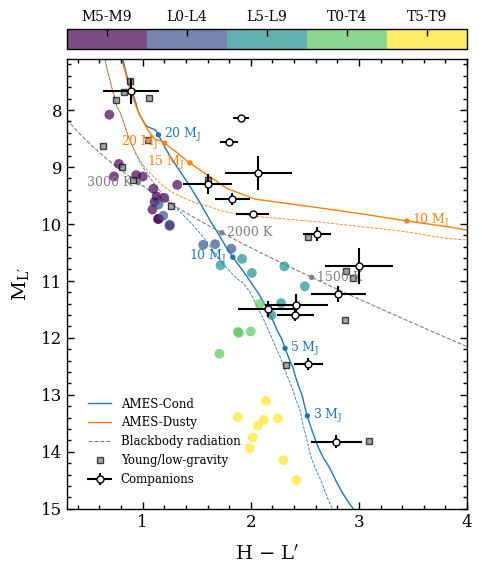
The plot_color_magnitude function returned the Figure object of the plot. The functionalities of Matplotlib can be used for further customization of the plot. For example, the axes of the plot are stored at the axes attribute of Figure.
[19]:
print(fig.axes[0])
Axes(0,0;1x0.9375)