Synthetic photometry

In this tutorial, we will compute the synthetic MKO J band flux from an IRTF spectrum of Jupiter.

Getting started

We start by importing the required Python packages.

import matplotlib.pyplot as plt
import numpy as np
from species import SpeciesInit
from species.core.box import create_box
from species.phot.syn_phot import SyntheticPhotometry
from species.plot.plot_spectrum import plot_spectrum

The species HDF5 database is initiated by creating an instance of the SpeciesInit class.

SpeciesInit()

==============
species v0.7.4
==============

Working folder: /Users/tomasstolker/applications/species/docs/tutorials
Creating species_config.ini... [DONE]

Configuration settings:
   - Database: /Users/tomasstolker/applications/species/docs/tutorials/species_database.hdf5
   - Data folder: /Users/tomasstolker/applications/species/docs/tutorials/data
   - Magnitude of Vega: 0.03
Creating species_database.hdf5... [DONE]
Creating data folder... [DONE]

Multiprocessing: mpi4py installed
Process number 1 out of 1...

<species.core.species_init.SpeciesInit at 0x1507b0610>

Jupiter spectrum

The spectrum of Jupiter that is used as an example is now downloaded from the IRTF website.

import urllib.request
urllib.request.urlretrieve('http://irtfweb.ifa.hawaii.edu/~spex/IRTF_Spectral_Library/Data/plnt_Jupiter.txt',
                           'data/plnt_Jupiter.txt')

('data/plnt_Jupiter.txt', <http.client.HTTPMessage at 0x150809850>)

The file contains the wavelength in \(\mu\)m, and the flux and uncertainty in W m\(^{-2}\) \(\mu\)m\(^-1\), which are also the units that are required by species. We can read the data with numpy.loadtxt.

wavelength, flux, error = np.loadtxt('data/plnt_Jupiter.txt', unpack=True)

Let’s create a SpectrumBox with the data.

spec_box = create_box('spectrum',
                      spectrum='irtf',
                      wavelength=wavelength,
                      flux=flux,
                      error=error,
                      name='jupiter')

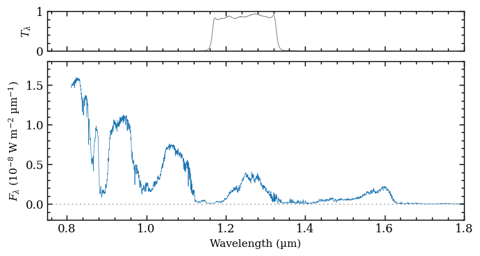
And pass the Box to the plot_spectrum function together with the filter name.

fig = plot_spectrum(boxes=[spec_box, ],
                    filters=['MKO/NSFCam.J'],
                    xlim=(0.75, 1.8),
                    ylim=(-2e-9, 1.8e-8),
                    offset=(-0.12, -0.05),
                    figsize=(7., 3.),
                    output=None)

-------------
Plot spectrum
-------------

Boxes:
   - SpectrumBox

Object type: planet
Quantity: flux density
Filter profiles: ['MKO/NSFCam.J']

Figure size: (7.0, 3.0)
Legend parameters: None
Include model name: False

The plot_spectrum function returned the Figure object of the plot. The functionalities of Matplotlib can be used for further customization of the plot. For example, the axes of the plot are stored at the axes attribute of Figure.

fig.axes

[<Axes: xlabel='Wavelength (μm)', ylabel='$F_\\lambda$ (10$^{-8}$ W m$^{-2}$ μm$^{-1}$)'>,
 <Axes: ylabel='$T_\\lambda$'>]

Synthetic flux and magnitude

Next, we use the SyntheticPhotometry class to calculate the flux and magnitude for the MKO/NSFCam.J filter. We first create and instance of SyntheticPhotometry with the filter name from the SVO website.

synphot = SyntheticPhotometry('MKO/NSFCam.J')

Downloading data from 'https://archive.stsci.edu/hlsps/reference-atlases/cdbs/current_calspec/alpha_lyr_stis_011.fits' to file '/Users/tomasstolker/applications/species/docs/tutorials/data/alpha_lyr_stis_011.fits'.
100%|████████████████████████████████████████| 288k/288k [00:00<00:00, 158MB/s]

Adding spectrum: VegaReference: Bohlin et al. 2014, PASP, 126
URL: https://ui.adsabs.harvard.edu/abs/2014PASP..126..711B/abstract

The average \(J\)-band flux is calculated with the spectrum_to_flux method. The error on the synthetic flux is estimated with Monte Carlo sampling of the input spectrum.

j_flux = synphot.spectrum_to_flux(wavelength, flux, error=error)
print(f'Flux (W m-2 um-1) = {j_flux[0]:.2e} +/- {j_flux[1]:.2e}')

Flux (W m-2 um-1) = 1.80e-09 +/- 8.87e-14

Similarly, we calculate the synthetic magnitude with the spectrum_to_magnitude method. Also the absolute magnitude can be calculated by providing the distance and uncertainty (set to None in the example). In species, the magnitude is defined relative to Vega, which is set in the configuration file by default to a magnitude of 0.03 in all filters. For the selected \(J\)-band filter, Jupiter has a magnitude of 0.59 so the planet is comparable in brightness to Vega.

j_mag, _ = synphot.spectrum_to_magnitude(wavelength, flux, error=error, distance=None)
print(f'Apparent magnitude = {j_mag[0]:.2f} +/- {j_mag[1]:.2e}')

Apparent magnitude = 0.58 +/- 5.16e-05