Working with evolutionary models
In this tutorial, we will work with data from an evolutionary model. We will extract an isochrone and cooling track by interpolating the data at a fixed age and mass, respectively. We will also compute synthetic photometry for a given age and mass by using the associated grid with model spectra.
Getting started
We start by importing matplotlib, numpy, and species.
[1]:
import matplotlib.pyplot as plt
import numpy as np
from species import SpeciesInit
from species.data.database import Database
from species.read.read_isochrone import ReadIsochrone
from species.plot.plot_spectrum import plot_spectrum
from species.plot.plot_color import plot_color_magnitude
Next, we initiate the workflow by calling the SpeciesInit class. This will create both the HDF5 database and the configuration file in the working folder.
[2]:
SpeciesInit()
=======
species
=======

Version: 0.9.1.dev64+g1d42feb.d20250418
Working folder: /Users/tomasstolker/applications/species/docs/tutorials

Creating species_config.ini... [DONE]
Creating species_database.hdf5... [DONE]
Creating data folder... [DONE]

Configuration settings:
   - Database: species_database.hdf5
   - Data folder: data
   - Magnitude of Vega: 0.03

Multiprocessing: mpi4py not installed
[2]:
<species.core.species_init.SpeciesInit at 0x12735ec30>
Now we will create and instance of Database that will provide read and write access to the HDF5 database where all the data will be stored.
[3]:
database = Database()
There are several evolutionary models supported by species. In this example, we will use the ATMO models that can be added with the add_isochrones method of Database. See the documentation of this method for a description of all the parameters and a list of other evolutionary models
that are supported.
With model='atmo', it will download and add both the chemical equilibrium and weak/strong non-equilibrium models of ATMO, including the magnitudes for MKO, WISE, and Spitzer filters.
[4]:
database.add_isochrones(model='atmo')
Downloading data from 'https://home.strw.leidenuniv.nl/~stolker/species/atmo_evolutionary_tracks.tgz' to file '/Users/tomasstolker/applications/species/docs/tutorials/data/atmo_evolutionary_tracks.tgz'.
------------------
Add isochrone grid
------------------

Evolutionary model: atmo
File name: None
Database tag: None
100%|█████████████████████████████████████| 9.98M/9.98M [00:00<00:00, 24.9GB/s]
Unpacking ATMO isochrones (9.6 MB)...
 [DONE]
Adding isochrones: ATMO equilibrium chemistry... [DONE]
Database tag: atmo-ceq
Adding isochrones: ATMO non-equilibrium chemistry (weak)... [DONE]
Database tag: atmo-neq-weak
Adding isochrones: ATMO non-equilibrium chemistry (strong)... [DONE]
Database tag: atmo-neq-strong
Extracting an isochrone
We can now read the evolutionary data from the database by creating an instance of ReadIsochrone and providing the tag by which the data was stored in the database with add_isochrones. We will use the ATMO CEQ isochrones which were calculated with a cloudless,
chemical-equilibrium atmosphere as boundary condition of the interior structure.
[5]:
read_iso = ReadIsochrone(tag='atmo-ceq')
-------------------
Read isochrone grid
-------------------

Database tag: atmo-ceq
Create regular grid: False

Setting 'extra_param' attribute: None
The get_filters method can be used to check for which filters there are magnitudes included with the isochrone grid.
[6]:
print(read_iso.get_filters())
['MKO_Y', 'MKO_J', 'MKO_H', 'MKO_K', 'MKO_Lp', 'MKO_Mp', 'W1', 'W2', 'W3', 'W4', 'IRAC_CH1', 'IRAC_CH2']
The ReadIsochrone has several functionalities (see link for a complete list of methods and parameters). For example, get_isochrone can be used to interpolate the evolutionary data at a fixed age and a range of masses. We can also optionally interpolate the magnitudes for
any of the filters that are included with the grid. For this, we need to use one of the filter names from get_filters as arguments for filter_mag and/or filters_color. Setting masses=None would select the masses at the nearest age point in the grid, but here we interpolate to a specified array of masses between 5 and 30 \(M_\mathrm{J}\).
[7]:
iso_box = read_iso.get_isochrone(age=50.,
                                 masses=np.linspace(5., 30., 50),
                                 filter_mag='MKO_H',
                                 filters_color=('MKO_K', 'MKO_Mp'))
The isochrone that is returned by get_isochrone is stored in an IsochroneBox. We can use the open_box method on any Box object to have a look at the content. Let’s have a look!
[8]:
iso_box.open_box()
Opening IsochroneBox...
model = atmo-ceq
age = 50.0
mass = [ 5.          5.51020408  6.02040816  6.53061224  7.04081633  7.55102041
  8.06122449  8.57142857  9.08163265  9.59183673 10.10204082 10.6122449
 11.12244898 11.63265306 12.14285714 12.65306122 13.16326531 13.67346939
 14.18367347 14.69387755 15.20408163 15.71428571 16.2244898  16.73469388
 17.24489796 17.75510204 18.26530612 18.7755102  19.28571429 19.79591837
 20.30612245 20.81632653 21.32653061 21.83673469 22.34693878 22.85714286
 23.36734694 23.87755102 24.3877551  24.89795918 25.40816327 25.91836735
 26.42857143 26.93877551 27.44897959 27.95918367 28.46938776 28.97959184
 29.48979592 30.        ]
teff = [ 721.86883896  764.57027946  804.235953    842.95432034  882.84151727
  921.98619473  958.93210586  994.73704115 1029.92588519 1067.96372949
 1106.67897556 1147.33026851 1198.45529003 1260.43331553 1363.11420439
 1472.83230803 1617.92858023 1760.8231806  1813.17009033 1889.334219
 1879.85432636 1834.99389221 1799.22369916 1769.50810461 1771.96572698
 1767.71477687 1782.90606587 1793.47315689 1806.33162875 1828.78456772
 1850.39163135 1870.48328275 1896.0853675  1918.71211965 1937.26191204
 1955.27393389 1973.98793885 1995.42568929 2018.19784074 2039.12525831
 2058.71022849 2078.54206978 2097.49090064 2116.67105469 2136.32670732
 2155.58375501 2173.89884328 2192.42995021 2211.48579453 2229.89759467]
log_lum = [-5.41371778 -5.31622851 -5.22771143 -5.14314577 -5.06258161 -4.98903519
 -4.92125201 -4.85530551 -4.79456264 -4.73267812 -4.670937   -4.60455143
 -4.52378449 -4.42996884 -4.27515212 -4.12024269 -3.92740233 -3.73578295
 -3.67528675 -3.58214078 -3.60397197 -3.6720226  -3.72794449 -3.77438153
 -3.7782386  -3.79191823 -3.77963507 -3.77304637 -3.76301631 -3.74184972
 -3.72102002 -3.70259369 -3.67796286 -3.65487565 -3.63656702 -3.61986933
 -3.6026895  -3.58242073 -3.56078997 -3.54113682 -3.52269394 -3.50399963
 -3.48640064 -3.46835371 -3.44968838 -3.43151958 -3.4144475  -3.397081
 -3.37910409 -3.36175976]
logg = [3.91450488 3.95625516 3.99460994 4.03047857 4.06321037 4.0937148
 4.12198915 4.14923347 4.17417153 4.19763102 4.21898199 4.23913284
 4.25492648 4.26684386 4.26610532 4.26287235 4.24276705 4.22553257
 4.23168913 4.22510968 4.25271621 4.29185849 4.32860484 4.3585908
 4.377861   4.40044976 4.41580949 4.43147725 4.44484924 4.45724564
 4.46838284 4.47939863 4.48795647 4.49615631 4.50508925 4.51419893
 4.52252945 4.53067783 4.53850263 4.54584983 4.55283193 4.55949444
 4.56568849 4.57174407 4.57772068 4.58325312 4.58838503 4.59336647
 4.59841535 4.6030679 ]
radius = [1.22634636 1.22753979 1.22783819 1.22760209 1.22742734 1.22776561
 1.22772595 1.22738062 1.22734885 1.2282214  1.22955219 1.23175593
 1.23793487 1.24930117 1.27711442 1.30939272 1.36770505 1.42053192
 1.4361132  1.4738039  1.45165728 1.4121864  1.37408114 1.34906096
 1.33947336 1.32404358 1.31920399 1.31365555 1.31080463 1.30937839
 1.30913789 1.30887974 1.31183537 1.3150066  1.31657009 1.31768751
 1.31961664 1.3215143  1.32351405 1.32604641 1.32884112 1.33186175
 1.33547219 1.33893247 1.34222168 1.34598985 1.35038226 1.35464331
 1.35853004 1.36281436]
filter_mag = MKO_H
magnitude = [16.53152285 16.21318631 15.92709625 15.65304799 15.39587278 15.15250773
 14.92645147 14.70811628 14.50139514 14.28215217 14.05840121 13.82493535
 13.52640345 13.1886765  12.65017532 12.16664833 11.69178323 11.19706906
 11.06222237 10.85586905 10.9031873  11.05273741 11.174994   11.2801804
 11.2876645  11.31689938 11.28676543 11.2708122  11.24808376 11.20018426
 11.15319863 11.11254588 11.05900513 11.00734693 10.96638537 10.92958662
 10.89205995 10.84807543 10.80122031 10.75869777 10.71870971 10.67814553
 10.64008523 10.60101497 10.56073625 10.5217359  10.48517582 10.44803012
 10.40934427 10.37200454]
filters_color = ('MKO_K', 'MKO_Mp')
color = [4.03652244 3.81032657 3.60928213 3.41503467 3.24028587 3.08869007
 2.95010238 2.81166962 2.69398154 2.57083685 2.44469743 2.31256384
 2.14313272 1.93106435 1.55966966 1.18264806 0.81071129 0.40330066
 0.33800932 0.28562866 0.29104786 0.35211882 0.37301101 0.4383164
 0.43684004 0.4416469  0.41163661 0.39821753 0.3880204  0.35296705
 0.32187728 0.30385083 0.29072711 0.26761759 0.24869116 0.24050399
 0.23753804 0.22481371 0.21015658 0.20217403 0.19841845 0.19626681
 0.19899088 0.19880644 0.19467216 0.19383706 0.19930032 0.20309515
 0.20482051 0.20962997]
The attributes from a Box can be simply extracted as usual for a Python object. For example, to extract the age at which the isochrone was interpolated:
[9]:
print(iso_box.age)
50.0
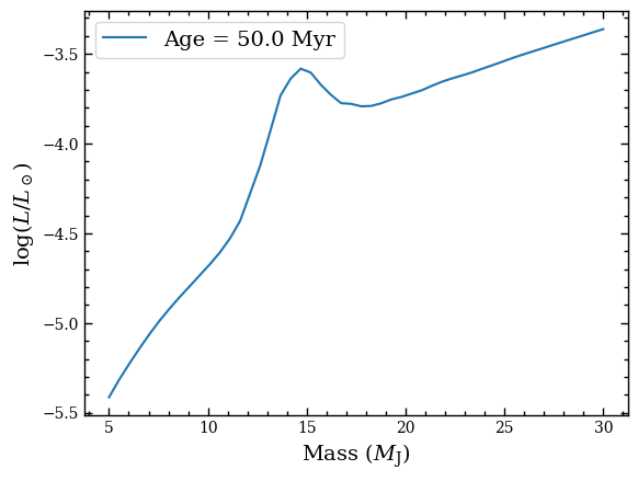
Let’s create a plot of the bolometric luminosity as function of mass.
[10]:
plt.plot(iso_box.mass, iso_box.log_lum, label=f'Age = {iso_box.age} Myr')
plt.xlabel(r'Mass ($M_\mathrm{J}$)', fontsize=14)
plt.ylabel(r'$\log(L/L_\odot)$', fontsize=14)
plt.legend(fontsize=14)
plt.show()
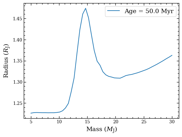
We can also plot the radius as function of mass.
[11]:
plt.plot(iso_box.mass, iso_box.radius, label=f'Age = {iso_box.age} Myr')
plt.xlabel(r'Mass ($M_\mathrm{J}$)', fontsize=14)
plt.ylabel(r'Radius ($R_\mathrm{J}$)', fontsize=14)
plt.legend(fontsize=14)
plt.show()
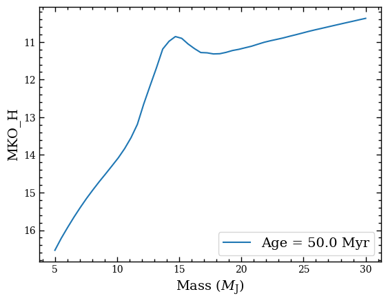
And finally let’s plot the absolute (i.e. at 10 pc) MKO \(H\)-band magnitude that we had selected.
[12]:
plt.plot(iso_box.mass, iso_box.magnitude, label=f'Age = {iso_box.age} Myr')
plt.xlabel(r'Mass ($M_\mathrm{J}$)', fontsize=14)
plt.ylabel(iso_box.filter_mag, fontsize=14)
plt.gca().invert_yaxis()
plt.legend(fontsize=14)
plt.show()
Extracting a cooling track
Similarly to extracting an isochrone, we can extract a cooling track with the get_cooling_track method, which will interpolate the evolutionary data at a fixed mass and a range of ages. Instead of providing an numpy array with ages, we can also set the argument of ages to None. In that case it use the ages that are available in the original data.
[10]:
cooling_box = read_iso.get_cooling_track(mass=10.,
                                         ages=None,
                                         filters_color=None,
                                         filter_mag=None)
The cooling track that is returned by get_cooling_track is stored in a CoolingBox. Let’s have a look at the content by again using the open_box method.
[11]:
cooling_box.open_box()
Opening CoolingBox...
model = atmo-ceq
mass = 10.0
age = [1.00000000e+00 1.26638017e+00 1.60371874e+00 2.03091762e+00
 2.57191381e+00 3.25702066e+00 4.12462638e+00 5.22334507e+00
 6.61474064e+00 8.37677640e+00 1.06081836e+01 1.34339933e+01
 1.70125428e+01 2.15443469e+01 2.72833338e+01 3.45510729e+01
 4.37547938e+01 5.54102033e+01 7.01703829e+01 8.88623816e+01
 1.12533558e+02 1.42510267e+02 1.80472177e+02 2.28546386e+02
 2.89426612e+02 3.66524124e+02 4.64158883e+02 5.87801607e+02
 7.44380301e+02 9.42668455e+02 1.19377664e+03 1.51177507e+03
 1.91448198e+03 2.42446202e+03 3.07029063e+03 3.88815518e+03
 4.92388263e+03 6.23550734e+03 7.89652287e+03 1.00000000e+04]
teff = [2309.92136414 2271.31843036 2227.60151094 2175.22268751 2113.25214823
 2045.29126453 1973.17836919 1895.94171811 1811.46845225 1723.32054156
 1634.65913374 1551.31030152 1459.23911948 1366.5750378  1287.77172299
 1211.22247039 1136.43302722 1064.724456    998.14220538  934.54155053
  870.8850384   807.72649858  749.53849188  697.6452082   651.37431096
  607.49484068  565.24890764  528.5033357   496.78042792  465.15856661
  435.45984711  408.48777861  384.35501994  362.15257628  343.71280978
  329.16168267  313.23919179  297.47716449  282.65774635  266.98078617]
log_lum = [-2.7647569  -2.85209906 -2.94259586 -3.03868041 -3.14100542 -3.24690055
 -3.35554457 -3.4680984  -3.58740346 -3.71078282 -3.83587559 -3.95736211
 -4.09218657 -4.23069065 -4.35652886 -4.48381341 -4.61367678 -4.74439666
 -4.87263193 -5.00190875 -5.13836696 -5.28140619 -5.42227616 -5.55683473
 -5.68536544 -5.81526128 -5.94846254 -6.07250345 -6.18738091 -6.30858479
 -6.42957971 -6.5469225  -6.65859787 -6.76796922 -6.86418136 -6.9454616
 -7.03789868 -7.13374161 -7.22885778 -7.33443872]
logg = [3.5898014  3.64784439 3.70452924 3.75916928 3.8112298  3.86034055
 3.90650505 3.94965859 3.98966366 4.02627813 4.0596115  4.09026099
 4.11813707 4.14311462 4.16568022 4.18643917 4.20549936 4.22302154
 4.23909491 4.25393916 4.26759116 4.27990516 4.29098952 4.30107731
 4.31037243 4.31906749 4.32716038 4.33472509 4.3419371  4.34881221
 4.35535939 4.36162777 4.36767451 4.37358752 4.37945448 4.38548586
 4.39168685 4.39792049 4.40419566 4.41048637]
radius = [2.52447902 2.36127149 2.21205989 2.07714109 1.95624733 1.84866899
 1.7529447  1.66795061 1.59284657 1.52707369 1.46956656 1.41860597
 1.37378998 1.33484008 1.30060555 1.26988667 1.2423234  1.2175119
 1.19518832 1.17493574 1.15661369 1.14033321 1.12587433 1.11287493
 1.10103001 1.09006398 1.07995542 1.07059103 1.06173891 1.05336863
 1.04545879 1.03794145 1.03074083 1.02374783 1.01685565 1.00981842
 1.00263439 0.99546417 0.98829787 0.98116589]
filter_mag = None
magnitude = None
filters_color = None
color = None
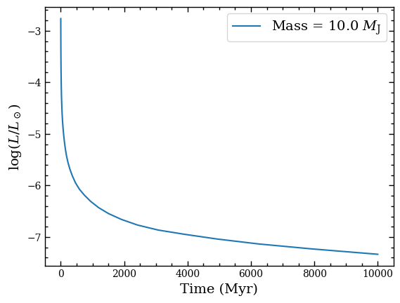
We can create a plot of the bolometric luminosity as function of time by selecting the respective attributes in the Box object.
[15]:
plt.plot(cooling_box.age, cooling_box.log_lum, label=f'Mass = {cooling_box.mass}'+r' $M_\mathrm{J}$')
plt.xlabel(r'Time (Myr)', fontsize=14)
plt.ylabel(r'$\log(L/L_\odot)$', fontsize=14)
plt.legend(fontsize=14)
plt.show()
Synthetic photometry from model spectra
As we saw earlier, magnitudes are available with some evolutionary models for some filters. If we want to calculate synthetic photometry for any arbitrary filter from the SVO Filter Profile Service, we can use the get_photometry method from ReadIsochrone. We simply need to provide the age, mass, distance, and name of the filter. For this example, we use the JWST/NIRCAM F360M filter.
The method selects automatically the atmospheric model that is associated with the evolutionary model (the argument of atmospheric_model is by default set to None) and downloads the data if not present in the data_folder. It then interpolates the grid of spectra at the bulk and atmospheric parameters for the requested age and mass, and uses the filter profile for the computation of the synthetic photometry.
[12]:
phot_box = read_iso.get_photometry(age=100., mass=20., distance=20., filter_name='JWST/NIRCam.F360M')
/Users/tomasstolker/applications/species/species/read/read_model.py:150: UserWarning: The 'atmo-ceq' model spectra are not present in the database. Will try to add the model grid. If this does not work (e.g. currently without an internet connection), then please use the 'add_model' method of 'Database' to add the grid of spectra at a later moment.
  warnings.warn(
Downloading data from 'https://home.strw.leidenuniv.nl/~stolker/species/atmo-ceq.tgz' to file '/Users/tomasstolker/applications/species/docs/tutorials/data/atmo-ceq.tgz'.
-------------------------
Add grid of model spectra
-------------------------

Database tag: atmo-ceq
Model name: ATMO CEQ
100%|████████████████████████████████████████| 476M/476M [00:00<00:00, 313GB/s]
SHA256 hash of downloaded file: bab2dc6920d9358bd0a554b9d5554b09e5885fec2daf91ee11ccf340c310fcbf
Use this value as the 'known_hash' argument of 'pooch.retrieve' to ensure that the file hasn't changed if it is downloaded again in the future.
Unpacking 231/231 model spectra from ATMO CEQ (455 MB)...data/atmo-ceq
data/atmo-ceq.tgz
 [DONE]

Please cite Phillips et al. (2020) when using ATMO CEQ in a publication
Reference URL: https://ui.adsabs.harvard.edu/abs/2020A%26A...637A..38P

Wavelength range (um) = 0.2 - 6000
Sampling (lambda/d_lambda) = 10000
Teff range (K) = 200 - 3000

Adding ATMO CEQ model spectra... data/atmo-ceq/atmo-ceq_teff_900_logg_5.5_spec.dat

Grid points stored in the database:
   - Teff = [ 200.  250.  300.  350.  400.  450.  500.  550.  600.  700.  800.  900.
 1000. 1100. 1200. 1300. 1400. 1500. 1600. 1700. 1800. 1900. 2000. 2100.
 2200. 2300. 2400. 2500. 2600. 2700. 2800. 2900. 3000.]
   - log(g) = [2.5 3.  3.5 4.  4.5 5.  5.5]

Number of grid points per parameter:
   - teff: 33
   - logg: 7

Number of stored grid points: 231
Number of interpolated grid points: 0
Number of missing grid points: 0
Downloading data from 'https://archive.stsci.edu/hlsps/reference-atlases/cdbs/current_calspec/alpha_lyr_stis_011.fits' to file '/Users/tomasstolker/applications/species/docs/tutorials/data/alpha_lyr_stis_011.fits'.
100%|████████████████████████████████████████| 288k/288k [00:00<00:00, 114MB/s]
Adding spectrum: Vega
Reference: Bohlin et al. 2014, PASP, 126
URL: https://ui.adsabs.harvard.edu/abs/2014PASP..126..711B/abstract
The get_photometry method returns a PhotometryBox that contains both the magnitude and flux density. Let’s use the open_box method to have a look at the content.
[13]:
phot_box.open_box()
Opening PhotometryBox...
name = atmo-ceq
sptype = None
wavelength = [3.62605786956827]
flux = [(3.014535553469553e-16, None)]
app_mag = [(13.266606538521108, None)]
abs_mag = [(11.761456560201202, None)]
filter_name = ['JWST/NIRCam.F360M']
Extracting a model spectrum
A model spectrum, as previously used for calculating the synthetic photometry, can also be extracted. This can be useful for analyzing the spectral appearance as function of age and mass. We can use the get_spectrum method and specify the age, mass, and distance. Additionally we can set the wavelength range and the spectral resolution that is used to smooth the spectra to the instrument’s resolution. We will extract the spectra for 10, 20, and 30 \(M_\mathrm{J}\) at an age of 100 Myr.
[14]:
boxes = []
for mass in [10., 20., 30.]:
    model_box = read_iso.get_spectrum(age=100., mass=mass, distance=20., wavel_range=(0.8, 5.), spec_res=100.)
    boxes.append(model_box)
The get_spectrum method returns a ModelBox. We can again use the open_box method to have a look at the content of the first
ModelBox in the boxes list.
[15]:
boxes[0].open_box()
Opening ModelBox...
model = atmo-ceq
type = None
wavelength = [0.79998813 0.8000674  0.80014669 ... 4.99918732 4.9996827  5.00017813]
flux = [3.66925465e-18 3.67881491e-18 3.68855193e-18 ... 6.96597313e-17
 6.96252108e-17 6.95901196e-17]
parameters = {'teff': 904.1733101126721, 'logg': 4.26009016659564, 'radius': 1.166674078951012, 'distance': 20.0, 'luminosity': 8.655066224443543e-06, 'mass': 9.99479099661175}
quantity = flux
contribution = None
bol_flux = None
spec_res = 100.0
The spectra can be easily plotted by passing the list of Box objects to the plot_spectrum function. Alternatively, one can select the wavelength and flux attributes from a ModelBox object and use
Matplotlib directly. Let’s have a look at the extracted spectrum!
[20]:
fig = plot_spectrum(boxes=boxes,
                    figsize=(5, 3),
                    legend={'loc': 'upper right', 'fontsize': 8.},
                    xlim=(0.8, 5.),
                    ylim=(2e-18, 1e-13),
                    scale=('linear', 'log'),
                    leg_param=['mass', 'luminosity', 'teff', 'radius'])
Plotting spectrum...
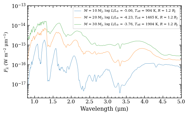
[DONE]
Computing color-magnitude tracks
Another method that is available for computing synthetic magnitudes, are the get_color_magnitude and get_color_color methods. In contrast to
get_photometry, we can specify an array with masses, and also the filters for the color and absolute magnitude. In this example, we set the argument of masses to None such that the mass points from the original grid are used that are closest to an age of 100 Myr.
We can specify any of the filters from the SVO Filter Profile Service as arguments for filters_color and filter_mag, since the photometry will be computed from the model spectra instead of extracted from the evolutionary grid. The method selects automatically the associated grid of model spectra and would download the data if not yet present in the data_folder.
[16]:
color_mag_box = read_iso.get_color_magnitude(age=100.,
                                             masses=None,
                                             filters_color=('JWST/MIRI.F560W', 'JWST/MIRI.F770W'),
                                             filter_mag='JWST/MIRI.F560W')
The get_color_magnitude method returns a ColorMagBox that contains all the data. Let’s have a look at its content with open_box.
[17]:
color_mag_box.open_box()
Opening ColorMagBox...
library = atmo-ceq
iso_tag = atmo-ceq
object_type = model
filters_color = ('JWST/MIRI.F560W', 'JWST/MIRI.F770W')
filter_mag = JWST/MIRI.F560W
color = [1.22305127 0.85480619 0.61034349 0.46349432 0.37319144 0.32106343
 0.29336056 0.25544585 0.22232437 0.16981534 0.12716618 0.08191179
 0.03221113 0.07575717 0.0408115  0.03282496 0.0327196  0.03386685
 0.0379404  0.04432713 0.05124139 0.06583403 0.0770041  0.09417916
 0.11016986 0.12787793 0.1420482  0.1535341  0.16325056 0.16971112
 0.1728354  0.17588333 0.17340426 0.17097304 0.16756559 0.16145802
 0.15603247 0.14939534 0.14141529 0.13439619 0.12768109 0.1210119
 0.11527149 0.11024621 0.10535235 0.10081233 0.09684413 0.09321272
 0.08993073 0.08696283 0.08422933 0.08170247 0.07940232 0.07722597
 0.07513635 0.07319228 0.07138914 0.06969032 0.06813241 0.06666673
 0.06540623 0.06415467 0.06302139 0.06193457 0.06090045 0.05991887
 0.05899907 0.05810653 0.05721747 0.05637178 0.05557424 0.05480974
 0.05407361 0.05336662 0.05268477 0.05203301]
magnitude = [19.03442901 17.3308523  16.01680868 15.17866781 14.57379637 14.10825348
 13.64313857 13.27577708 12.97711335 12.66714535 12.37890678 12.01029346
 11.19648293 10.51007624 10.83805222 11.07170853 11.08915331 11.03985657
 10.96999791 10.89754622 10.82173021 10.73957721 10.67105543 10.60506587
 10.53578961 10.4702035  10.4126034  10.3522146  10.2942058  10.2360866
 10.1772606  10.11992047 10.05848352 10.00047606  9.94387958  9.88507284
  9.82888929  9.77169661  9.71339334  9.65891656  9.60359734  9.54491644
  9.49108974  9.44106232  9.38932537  9.33873806  9.29189375  9.24706151
  9.20337274  9.16031429  9.11893441  9.07905063  9.04101609  9.00420571
  8.96869029  8.93431907  8.90120221  8.86891154  8.83795208  8.80776873
  8.77979041  8.75016305  8.72271805  8.69580378  8.66950165  8.64384243
  8.61892518  8.594599    8.57104471  8.54795899  8.52544274  8.50330719
  8.48149494  8.46004967  8.43890002  8.41814415]
names = None
sptype = None
mass = [ 0.52378276  1.04756551  2.09513103  3.14269654  4.19026206  5.23782757
  6.28539309  7.3329586   8.38052412  9.42808963 10.47565515 11.52322066
 12.57078618 13.61835169 14.66591721 15.71348272 16.76104823 17.80861375
 18.85617926 19.90374478 20.95131029 21.99887581 23.04644132 24.09400684
 25.14157235 26.18913787 27.23670338 28.2842689  29.33183441 30.37939993
 31.42696544 32.47453095 33.52209647 34.56966198 35.6172275  36.66479301
 37.71235853 38.75992404 39.80748956 40.85505507 41.90262059 42.9501861
 43.99775162 45.04531713 46.09288265 47.14044816 48.18801367 49.23557919
 50.2831447  51.33071022 52.37827573 53.42584125 54.47340676 55.52097228
 56.56853779 57.61610331 58.66366882 59.71123434 60.75879985 61.80636536
 62.85393088 63.90149639 64.94906191 65.99662742 67.04419294 68.09175845
 69.13932397 70.18688948 71.234455   72.28202051 73.32958603 74.37715154
 75.42471706 76.47228257 77.51984808 78.5674136 ]
radius = [1.07904507 1.14021908 1.1716395  1.17916743 1.18267947 1.18234894
 1.17941627 1.17542196 1.17108353 1.16725245 1.16553525 1.17313138
 1.22661116 1.30784146 1.23860974 1.19506142 1.17922427 1.17152071
 1.16693897 1.16406892 1.16243355 1.16326991 1.16320022 1.16398137
 1.1654034  1.16752663 1.17009763 1.1731298  1.17652692 1.18033408
 1.18446036 1.1888885  1.19373147 1.19897058 1.20452157 1.21039603
 1.21651376 1.2229402  1.22959482 1.23646496 1.24353968 1.25086333
 1.258366   1.26604744 1.27386113 1.28181197 1.2898484  1.29796845
 1.30613904 1.31439804 1.32269372 1.33104161 1.33943155 1.34785985
 1.35631085 1.36482463 1.37334495 1.3819219  1.39052997 1.39914585
 1.40726217 1.41640495 1.42504561 1.43366853 1.44228345 1.45088109
 1.45948849 1.46809576 1.47669858 1.48532386 1.49395381 1.50259519
 1.51125239 1.51990769 1.52857923 1.5372489 ]
The attributes from the ColorMagBox can be plotted manually or it can be directly provided as input to the plot_color_magnitude function. Similarly, a returned ColorColorBox from the get_color_color method of ReadIsochrone can be used as input to the plot_color_color function.
The plot_color_magnitude function requires a list of Box objects as input, which is provided as argument of boxes. In this example, we only include for simplicity only a single item in the list with boxes. We place also several labels at specific masses of the color-magnitude track that we
extracted from the ATMO CEQ models.
[23]:
fig = plot_color_magnitude(boxes=[color_mag_box],
                           mass_labels={'atmo-ceq': [(1., 'right'), (5., 'left'), (10., 'left'), (30., 'right')]},
                           label_x=r"F560W $-$ F770W",
                           label_y=r"M$_\mathrm{F560W}$",
                           xlim=(-0.5, 1.5),
                           legend={'loc': 'upper right', 'frameon': False, 'fontsize': 12.})
Plotting color-magnitude diagram...
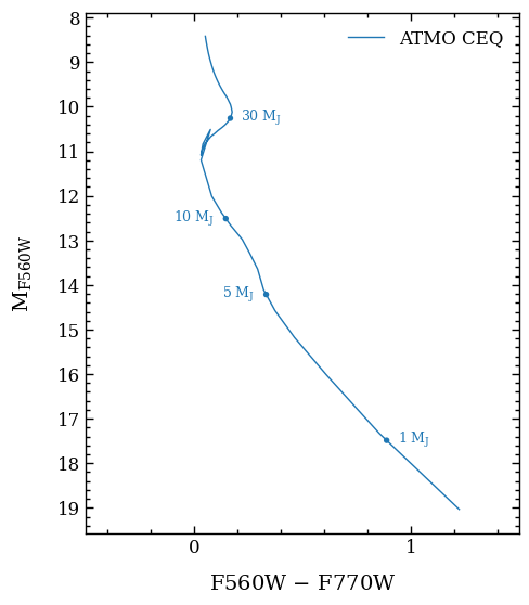
[DONE]
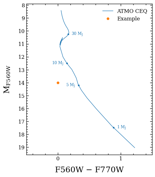
The plot_color_magnitude returned the Figure object of the plot. The functionalities of Matplotlib can be used for further customization of the plot. For example, the axes of the plot are stored at the axes attribute of Figure.
[24]:
fig.axes
[24]:
[<Axes: xlabel='F560W $-$ F770W', ylabel='M$_\\mathrm{F560W}$'>]
In this case the list of axes contains only a single item. As an example we will add an additional data point, update the legend, and increase the fontsize of the axis labels.
[25]:
fig.axes[0].plot(0., 14, 'o', color='tab:orange', ms=5, label='Example')
fig.axes[0].legend(frameon=False, fontsize=12)
fig.axes[0].xaxis.label.set_fontsize(18.)
fig.axes[0].yaxis.label.set_fontsize(18.)
To show the updated figure, we simply call the Figure object of the plot. To save the plot to a file, the savefig method of the figure can be used.
[26]:
fig
[26]:
Converting contrast into mass
The contrast_to_mass method of ReadIsochrone can be used to convert a list or array with companion-to-star contrast values into masses of the companion. This feature can be useful for converting a contrast curve (i.e. detection limits for point sources) into mass limits as function of separation from the star. Or, to estimate the mass of a companion from a measured brightness contrast with its star.
We can either select one of the filters with pre-calculated magnitudes that come with the isochrone grid (i.e., those returned by get_filters) or any of the filters from the SVO Filter Profile Service.
For example, let’s select the MKO_H filter that is include with the ATMO grid and interpolate the masses for a list of contrast values that are provided as magnitudes.
[18]:
masses = read_iso.contrast_to_mass(age=20.,
                                   distance=50.,
                                   filter_name='MKO_H',
                                   star_mag=10.,
                                   contrast=[5.0, 7.5, 10.],
                                   use_mag=True)
print(masses)
The 'MKO_H' filter is found in the list of available filters from the isochrone data of 'atmo-ceq'.
The requested contrast values will be directly interpolated from the grid with pre-calculated magnitudes.
[12.18523169  6.5719161   3.0361701 ]
Alternatively, we can select a filter from the SVO Filter Profile Service. In this case, the function will use the associated model spectra for calculating and interpolating the synthetic photometry. In this example we will provide the contrast values as ratios instead of magnitudes, so we set use_mag=False.
[19]:
masses = read_iso.contrast_to_mass(age=20.,
                                   distance=50.,
                                   filter_name='JWST/NIRCam.F162M',
                                   star_mag=10.,
                                   contrast=[1e-2, 1e-3, 1e-4],
                                   use_mag=False)
print(masses)
The 'JWST/NIRCam.F162M' filter is not found in the list of available filters from the isochrone data of 'atmo-ceq'.
It will be tried to download the filter profile (if needed) and to use the associated atmospheric model spectra for calculating synthetic photometry.
[11.68030143  6.2010683   2.81440063]
/Users/tomasstolker/applications/species/species/read/read_model.py:1567: UserWarning: The set of model parameters {'teff': 3001.357148379523, 'logg': 4.455553724453863, 'radius': 2.526381394429854, 'distance': 50.0} is outside the grid range {'teff': (200.0, 3000.0), 'logg': (2.5, 5.5)} so returning a NaN.
  warnings.warn(
/Users/tomasstolker/applications/species/species/read/read_model.py:1567: UserWarning: The set of model parameters {'teff': 3006.482388036101, 'logg': 4.4562069114763485, 'radius': 2.5424416720662784, 'distance': 50.0} is outside the grid range {'teff': (200.0, 3000.0), 'logg': (2.5, 5.5)} so returning a NaN.
  warnings.warn(
/Users/tomasstolker/applications/species/species/read/read_model.py:1567: UserWarning: The set of model parameters {'teff': 3011.408951792053, 'logg': 4.456811598156431, 'radius': 2.558493215446333, 'distance': 50.0} is outside the grid range {'teff': (200.0, 3000.0), 'logg': (2.5, 5.5)} so returning a NaN.
  warnings.warn(
/Users/tomasstolker/applications/species/species/read/read_model.py:1567: UserWarning: The set of model parameters {'teff': 3016.267586113234, 'logg': 4.457442944709719, 'radius': 2.5743185127516264, 'distance': 50.0} is outside the grid range {'teff': (200.0, 3000.0), 'logg': (2.5, 5.5)} so returning a NaN.
  warnings.warn(
/Users/tomasstolker/applications/species/species/read/read_model.py:1567: UserWarning: The set of model parameters {'teff': 3021.073033921284, 'logg': 4.458036630627344, 'radius': 2.5901106044291575, 'distance': 50.0} is outside the grid range {'teff': (200.0, 3000.0), 'logg': (2.5, 5.5)} so returning a NaN.
  warnings.warn(
/Users/tomasstolker/applications/species/species/read/read_model.py:1567: UserWarning: The set of model parameters {'teff': 3025.8044035429903, 'logg': 4.45866077561258, 'radius': 2.6056736019935696, 'distance': 50.0} is outside the grid range {'teff': (200.0, 3000.0), 'logg': (2.5, 5.5)} so returning a NaN.
  warnings.warn(
Several warnings appeared because some of the effective temperatures from the ischrone data are outside the available range of the associated atmospheric model. Those magnitudes are set to NaN such that converting any contrast values into masses for objects in the 3000 K regime will not be possible. Any contrast values in that regime will be returned as NaN as well, which is not the case in this example.