Comparing photometric fluxes and model spectra
In this tutorial, we will compare the photometric fluxes of the brown dwarf companion PZ Tel B with a synthetic spectrum from the ATMO grid.
Initiating species
We start by importing species.
[1]:
from species import SpeciesInit
from species.data.database import Database
from species.read.read_model import ReadModel
from species.plot.plot_spectrum import plot_spectrum
from species.util.fit_util import get_residuals, multi_photometry
And initiating the workflow with the SpeciesInit class. This will create the configuration file and the HDF5 database.
[2]:
SpeciesInit()
=======
species
=======

Version: 0.9.1.dev64+g1d42feb.d20250418
Working folder: /Users/tomasstolker/applications/species/docs/tutorials

Creating species_config.ini... [DONE]
Creating species_database.hdf5... [DONE]
Creating data folder... [DONE]

Configuration settings:
   - Database: species_database.hdf5
   - Data folder: data
   - Magnitude of Vega: 0.03

Multiprocessing: mpi4py not installed
[2]:
<species.core.species_init.SpeciesInit at 0x119271d30>
Adding model spectra
We create now a Database object which is used for importing various data into the database.
[3]:
database = Database()
The spectra of ATMO are downloaded and added to the database with the add_model method of Database. This requires sufficient disk storage in the data_folder that is set in the configuration file. The full ATMO grid is downloaded but the teff_range parameter can be used to only import a
certain \(T_\mathrm{eff}\) range into the database.
[4]:
database.add_model('atmo', teff_range=(2500., 3000.))
Downloading data from 'https://home.strw.leidenuniv.nl/~stolker/species/atmo.tgz' to file '/Users/tomasstolker/applications/species/docs/tutorials/data/atmo.tgz'.
-------------------------
Add grid of model spectra
-------------------------

Database tag: atmo
Model name: ATMO
100%|█████████████████████████████████████| 21.1M/21.1M [00:00<00:00, 40.1GB/s]
Unpacking 42/231 model spectra from ATMO (21 MB)... [DONE]

Please cite Phillips et al. (2020) when using ATMO in a publication
Reference URL: https://ui.adsabs.harvard.edu/abs/2020A%26A...637A..38P

Wavelength range (um) = 0.2 - 2000
Sampling (lambda/d_lambda) = 1000
Teff range (K) = 2500.0 - 3000.0

Adding ATMO model spectra... data/atmo/atmo_teff_3000_logg_5.5_spec.npy

Grid points stored in the database:
   - Teff = [2500. 2600. 2700. 2800. 2900. 3000.]
   - log(g) = [2.5 3.  3.5 4.  4.5 5.  5.5]

Number of grid points per parameter:
   - teff: 6
   - logg: 7

Number of stored grid points: 42
Number of interpolated grid points: 0
Number of missing grid points: 0
Adding companion data
Next, we add the parallax and magnitudes of PZ Tel B to the database with the add_companion method. This will automatically download the required filter profiles and a flux-calibrated spectrum of Vega. These are used to convert the magnitudes into fluxes.
[5]:
database.add_companion('PZ Tel B', verbose=False)
Add companion: ['PZ Tel B']
Downloading data from 'https://archive.stsci.edu/hlsps/reference-atlases/cdbs/current_calspec/alpha_lyr_stis_011.fits' to file '/Users/tomasstolker/applications/species/docs/tutorials/data/alpha_lyr_stis_011.fits'.
100%|████████████████████████████████████████| 288k/288k [00:00<00:00, 322MB/s]
Adding spectrum: Vega
Reference: Bohlin et al. 2014, PASP, 126
URL: https://ui.adsabs.harvard.edu/abs/2014PASP..126..711B/abstract
Alternatively, the add_object method of Database can be used for manually adding magnitudes and spectra of an individual object. Before continuing, let’s check the content of the database.
[6]:
database.list_content()
---------------------
List database content
---------------------

- filters: <HDF5 group "/filters" (2 members)>
        - Gemini: <HDF5 group "/filters/Gemini" (2 members)>
                - NICI.ED286: <HDF5 dataset "NICI.ED286": shape (387, 2), type "<f8">
                        - det_type: energy
                        - det_type = energy
                - NIRI.H2S1v2-1-G0220: <HDF5 dataset "NIRI.H2S1v2-1-G0220": shape (129, 2), type "<f8">
                        - det_type: energy
                        - det_type = energy
        - Paranal: <HDF5 group "/filters/Paranal" (12 members)>
                - NACO.H: <HDF5 dataset "NACO.H": shape (23, 2), type "<f8">
                        - det_type: energy
                        - det_type = energy
                - NACO.J: <HDF5 dataset "NACO.J": shape (20, 2), type "<f8">
                        - det_type: energy
                        - det_type = energy
                - NACO.Ks: <HDF5 dataset "NACO.Ks": shape (27, 2), type "<f8">
                        - det_type: energy
                        - det_type = energy
                - NACO.Lp: <HDF5 dataset "NACO.Lp": shape (31, 2), type "<f8">
                        - det_type: energy
                        - det_type = energy
                - NACO.Mp: <HDF5 dataset "NACO.Mp": shape (18, 2), type "<f8">
                        - det_type: energy
                        - det_type = energy
                - NACO.NB405: <HDF5 dataset "NACO.NB405": shape (67, 2), type "<f8">
                        - det_type: energy
                        - det_type = energy
                - SPHERE.IRDIS_D_H23_2: <HDF5 dataset "SPHERE.IRDIS_D_H23_2": shape (113, 2), type "<f8">
                        - det_type: energy
                        - det_type = energy
                - SPHERE.IRDIS_D_H23_3: <HDF5 dataset "SPHERE.IRDIS_D_H23_3": shape (180, 2), type "<f8">
                        - det_type: energy
                        - det_type = energy
                - SPHERE.IRDIS_D_K12_1: <HDF5 dataset "SPHERE.IRDIS_D_K12_1": shape (175, 2), type "<f8">
                        - det_type: energy
                        - det_type = energy
                - SPHERE.IRDIS_D_K12_2: <HDF5 dataset "SPHERE.IRDIS_D_K12_2": shape (191, 2), type "<f8">
                        - det_type: energy
                        - det_type = energy
                - SPHERE.ZIMPOL_I_PRIM: <HDF5 dataset "SPHERE.ZIMPOL_I_PRIM": shape (189, 2), type "<f8">
                        - det_type: energy
                        - det_type = energy
                - SPHERE.ZIMPOL_R_PRIM: <HDF5 dataset "SPHERE.ZIMPOL_R_PRIM": shape (169, 2), type "<f8">
                        - det_type: energy
                        - det_type = energy
- models: <HDF5 group "/models" (1 members)>
        - atmo: <HDF5 group "/models/atmo" (4 members)>
                - flux: <HDF5 dataset "flux": shape (6, 7, 9249), type "<f8">
                - logg: <HDF5 dataset "logg": shape (7,), type "<f8">
                - teff: <HDF5 dataset "teff": shape (6,), type "<f8">
                - wavelength: <HDF5 dataset "wavelength": shape (9249,), type "<f8">
                - lambda/d_lambda = 1000
                - n_param = 2
                - parameter0 = teff
                - parameter1 = logg
- objects: <HDF5 group "/objects" (1 members)>
        - PZ Tel B: <HDF5 group "/objects/PZ Tel B" (3 members)>
                - Gemini: <HDF5 group "/objects/PZ Tel B/Gemini" (2 members)>
                        - NICI.ED286: <HDF5 dataset "NICI.ED286": shape (4,), type "<f8">
                                - n_phot: 1
                                - n_phot = 1
                        - NIRI.H2S1v2-1-G0220: <HDF5 dataset "NIRI.H2S1v2-1-G0220": shape (4,), type "<f8">
                                - n_phot: 1
                                - n_phot = 1
                - Paranal: <HDF5 group "/objects/PZ Tel B/Paranal" (12 members)>
                        - NACO.H: <HDF5 dataset "NACO.H": shape (4,), type "<f8">
                                - n_phot: 1
                                - n_phot = 1
                        - NACO.J: <HDF5 dataset "NACO.J": shape (4,), type "<f8">
                                - n_phot: 1
                                - n_phot = 1
                        - NACO.Ks: <HDF5 dataset "NACO.Ks": shape (4,), type "<f8">
                                - n_phot: 1
                                - n_phot = 1
                        - NACO.Lp: <HDF5 dataset "NACO.Lp": shape (4,), type "<f8">
                                - n_phot: 1
                                - n_phot = 1
                        - NACO.Mp: <HDF5 dataset "NACO.Mp": shape (4,), type "<f8">
                                - n_phot: 1
                                - n_phot = 1
                        - NACO.NB405: <HDF5 dataset "NACO.NB405": shape (4,), type "<f8">
                                - n_phot: 1
                                - n_phot = 1
                        - SPHERE.IRDIS_D_H23_2: <HDF5 dataset "SPHERE.IRDIS_D_H23_2": shape (4,), type "<f8">
                                - n_phot: 1
                                - n_phot = 1
                        - SPHERE.IRDIS_D_H23_3: <HDF5 dataset "SPHERE.IRDIS_D_H23_3": shape (4,), type "<f8">
                                - n_phot: 1
                                - n_phot = 1
                        - SPHERE.IRDIS_D_K12_1: <HDF5 dataset "SPHERE.IRDIS_D_K12_1": shape (4,), type "<f8">
                                - n_phot: 1
                                - n_phot = 1
                        - SPHERE.IRDIS_D_K12_2: <HDF5 dataset "SPHERE.IRDIS_D_K12_2": shape (4,), type "<f8">
                                - n_phot: 1
                                - n_phot = 1
                        - SPHERE.ZIMPOL_I_PRIM: <HDF5 dataset "SPHERE.ZIMPOL_I_PRIM": shape (4,), type "<f8">
                                - n_phot: 1
                                - n_phot = 1
                        - SPHERE.ZIMPOL_R_PRIM: <HDF5 dataset "SPHERE.ZIMPOL_R_PRIM": shape (4,), type "<f8">
                                - n_phot: 1
                                - n_phot = 1
                - parallax: <HDF5 dataset "parallax": shape (2,), type "<f8">
- spectra: <HDF5 group "/spectra" (1 members)>
        - calibration: <HDF5 group "/spectra/calibration" (1 members)>
                - vega: <HDF5 dataset "vega": shape (3, 9192), type "<f8">
We see the various groups, subgroups, datasets, and attributes that are stored in the HDF5 database.
Reading model spectra
Model spectra are read from the database by first creating an instance of ReadModel. The model name and optionally a wavelength range are provided as arguments.
[7]:
readmodel = ReadModel('atmo', wavel_range=(0.5, 10.))
Before extracting a spectrum, let’s check which parameters are required for the ATMO model spectra.
[8]:
readmodel.get_parameters()
[8]:
['teff', 'logg']
And also the parameter boundaries of the grid that is stored in the database.
[9]:
readmodel.get_bounds()
[9]:
{'teff': (np.float64(2500.0), np.float64(3000.0)),
 'logg': (np.float64(2.5), np.float64(5.5))}
The parameters are provided in a dictionary for which we have to make sure that chose values are within the grid boundaries. The radius (\(R_\mathrm{J}\)) and distance (pc) will scale the emitted spectrum to the observer. Without these values, the spectrum fluxes are provided at the surface of the atmosphere.
[10]:
model_param = {'teff': 2900., 'logg': 4.5, 'radius': 2.2, 'distance': 47.13}
We now use the get_model method of ReadModel to linearly interpolate the grid of spectra and store the extracted spectrum in a ModelBox. The spectrum is smoothed to a spectral resolution of \(R = 100\).
[11]:
modelbox = readmodel.get_model(model_param, spec_res=100., smooth=True)
Reading companion data
The photometric data of PZ Tel B are also read from the database and stored in an ObjectBox.
[12]:
objectbox = database.get_object(object_name='PZ Tel B')
----------
Get object
----------

Object name: PZ Tel B
Include photometry: True
Include spectra: True
Synthetic photometry for all filters
For comparison, we create synthetic photometry from the extracted ATMO spectrum for all filters of PZ Tel B. The synthetic fluxes are stored in a SynphotBox.
[13]:
synphot_box = multi_photometry(datatype='model',
                               spectrum='atmo',
                               filters=objectbox.filters,
                               parameters=model_param)
--------------------------
Calculate multi-photometry
--------------------------

Data type: model
Spectrum name: atmo

Parameters:
   - teff = 2900.00
   - logg = 4.50
   - radius = 2.20
   - distance = 47.13
   - log_lum_atm = -2.49
   - log_lum = -2.49
   - mass = 61.75

Magnitudes:
   - Gemini/NICI.ED286 = 11.82
   - Gemini/NIRI.H2S1v2-1-G0220 = 11.32
   - Paranal/NACO.H = 11.79
   - Paranal/NACO.J = 12.37
   - Paranal/NACO.Ks = 11.52
   - Paranal/NACO.Lp = 10.97
   - Paranal/NACO.Mp = 11.04
   - Paranal/NACO.NB405 = 10.89
   - Paranal/SPHERE.IRDIS_D_H23_2 = 11.82
   - Paranal/SPHERE.IRDIS_D_H23_3 = 11.58
   - Paranal/SPHERE.IRDIS_D_K12_1 = 11.59
   - Paranal/SPHERE.IRDIS_D_K12_2 = 11.33
   - Paranal/SPHERE.ZIMPOL_I_PRIM = 14.44
   - Paranal/SPHERE.ZIMPOL_R_PRIM = 16.96

Fluxes (W m-2 um-1):
   - Gemini/NICI.ED286 = 2.40e-14
   - Gemini/NIRI.H2S1v2-1-G0220 = 1.11e-14
   - Paranal/NACO.H = 2.20e-14
   - Paranal/NACO.J = 3.37e-14
   - Paranal/NACO.Ks = 1.11e-14
   - Paranal/NACO.Lp = 2.10e-15
   - Paranal/NACO.Mp = 8.16e-16
   - Paranal/NACO.NB405 = 1.71e-15
   - Paranal/SPHERE.IRDIS_D_H23_2 = 2.41e-14
   - Paranal/SPHERE.IRDIS_D_H23_3 = 2.54e-14
   - Paranal/SPHERE.IRDIS_D_K12_1 = 1.11e-14
   - Paranal/SPHERE.IRDIS_D_K12_2 = 1.09e-14
   - Paranal/SPHERE.ZIMPOL_I_PRIM = 2.11e-14
   - Paranal/SPHERE.ZIMPOL_R_PRIM = 4.10e-15
Opening Box objects
The open_box method can be used to view the content of any Box object. For example, the ModelBox contains several attributes, including the wavelengths and fluxes.
[14]:
modelbox.open_box()
Opening ModelBox...
model = atmo
type = None
wavelength = [ 0.49082927  0.49131575  0.49180271 ... 10.16291896 10.17299187
 10.18307476]
flux = [4.32979056e-15 4.44278351e-15 4.54287819e-15 ... 5.50293177e-17
 5.49825601e-17 5.49507556e-17]
parameters = {'teff': 2900.0, 'logg': 4.5, 'radius': 2.2, 'distance': 47.13, 'log_lum_atm': np.float64(-2.487198081818381), 'log_lum': np.float64(-2.487198081818381), 'mass': np.float64(61.74898371650208)}
quantity = flux
contribution = None
bol_flux = None
spec_res = 100.0
extra_out = None
Similarly, an ObjectBox contains a dictionary with the magnitudes and a dictionary with the fluxes.
[15]:
objectbox.open_box()
Opening ObjectBox...
name = PZ Tel B
filters = ['Gemini/NICI.ED286', 'Gemini/NIRI.H2S1v2-1-G0220', 'Paranal/NACO.H', 'Paranal/NACO.J', 'Paranal/NACO.Ks', 'Paranal/NACO.Lp', 'Paranal/NACO.Mp', 'Paranal/NACO.NB405', 'Paranal/SPHERE.IRDIS_D_H23_2', 'Paranal/SPHERE.IRDIS_D_H23_3', 'Paranal/SPHERE.IRDIS_D_K12_1', 'Paranal/SPHERE.IRDIS_D_K12_2', 'Paranal/SPHERE.ZIMPOL_I_PRIM', 'Paranal/SPHERE.ZIMPOL_R_PRIM']
mean_wavel = {'Gemini/NICI.ED286': np.float64(1.5841803431418238), 'Gemini/NIRI.H2S1v2-1-G0220': np.float64(2.2447142746110718), 'Paranal/NACO.H': np.float64(1.6588090664617747), 'Paranal/NACO.J': np.float64(1.265099894847529), 'Paranal/NACO.Ks': np.float64(2.144954491491888), 'Paranal/NACO.Lp': np.float64(3.8050282724280526), 'Paranal/NACO.Mp': np.float64(4.780970919324577), 'Paranal/NACO.NB405': np.float64(4.055862923806052), 'Paranal/SPHERE.IRDIS_D_H23_2': np.float64(1.5863509078883227), 'Paranal/SPHERE.IRDIS_D_H23_3': np.float64(1.6661442175885708), 'Paranal/SPHERE.IRDIS_D_K12_1': np.float64(2.1038552712775034), 'Paranal/SPHERE.IRDIS_D_K12_2': np.float64(2.255172356268582), 'Paranal/SPHERE.ZIMPOL_I_PRIM': np.float64(0.7843997176190827), 'Paranal/SPHERE.ZIMPOL_R_PRIM': np.float64(0.6278112553204571)}
filter_width = {'Gemini/NICI.ED286': np.float64(0.017525193213729695), 'Gemini/NIRI.H2S1v2-1-G0220': np.float64(0.035876346375876444), 'Paranal/NACO.H': np.float64(0.34479579328929977), 'Paranal/NACO.J': np.float64(0.24904070813234003), 'Paranal/NACO.Ks': np.float64(0.36972828247409306), 'Paranal/NACO.Lp': np.float64(0.6276348582389186), 'Paranal/NACO.Mp': np.float64(0.5952960574619803), 'Paranal/NACO.NB405': np.float64(0.06124789557254662), 'Paranal/SPHERE.IRDIS_D_H23_2': np.float64(0.05333096018675132), 'Paranal/SPHERE.IRDIS_D_H23_3': np.float64(0.055530714769082445), 'Paranal/SPHERE.IRDIS_D_K12_1': np.float64(0.10240523658303102), 'Paranal/SPHERE.IRDIS_D_K12_2': np.float64(0.11039405718538875), 'Paranal/SPHERE.ZIMPOL_I_PRIM': np.float64(0.16199089822589552), 'Paranal/SPHERE.ZIMPOL_R_PRIM': np.float64(0.14691237592187478)}
magnitude = {'Gemini/NICI.ED286': array([11.68,  0.14]), 'Gemini/NIRI.H2S1v2-1-G0220': array([11.39,  0.14]), 'Paranal/NACO.H': array([11.93,  0.14]), 'Paranal/NACO.J': array([12.47,  0.2 ]), 'Paranal/NACO.Ks': array([11.53,  0.07]), 'Paranal/NACO.Lp': array([11.04,  0.22]), 'Paranal/NACO.Mp': array([10.93,  0.03]), 'Paranal/NACO.NB405': array([10.94,  0.07]), 'Paranal/SPHERE.IRDIS_D_H23_2': array([11.78,  0.19]), 'Paranal/SPHERE.IRDIS_D_H23_3': array([11.65,  0.19]), 'Paranal/SPHERE.IRDIS_D_K12_1': array([11.56,  0.09]), 'Paranal/SPHERE.IRDIS_D_K12_2': array([11.29,  0.1 ]), 'Paranal/SPHERE.ZIMPOL_I_PRIM': array([15.16,  0.12]), 'Paranal/SPHERE.ZIMPOL_R_PRIM': array([17.84,  0.31])}
flux = {'Gemini/NICI.ED286': array([2.74086109e-14, 3.54399875e-15]), 'Gemini/NIRI.H2S1v2-1-G0220': array([1.03991914e-14, 1.34464024e-15]), 'Paranal/NACO.H': array([1.93752511e-14, 2.50526617e-15]), 'Paranal/NACO.J': array([3.07259575e-14, 5.69199382e-15]), 'Paranal/NACO.Ks': array([1.10414095e-14, 7.12359249e-16]), 'Paranal/NACO.Lp': array([1.97779118e-15, 4.03502853e-16]), 'Paranal/NACO.Mp': array([9.00005271e-16, 2.48712291e-17]), 'Paranal/NACO.NB405': array([1.63652876e-15, 1.05584019e-16]), 'Paranal/SPHERE.IRDIS_D_H23_2': array([2.50237615e-14, 4.40145471e-15]), 'Paranal/SPHERE.IRDIS_D_H23_3': array([2.38720055e-14, 4.19887118e-15]), 'Paranal/SPHERE.IRDIS_D_K12_1': array([1.13423556e-14, 9.41279698e-16]), 'Paranal/SPHERE.IRDIS_D_K12_2': array([1.12217121e-14, 1.03501979e-15]), 'Paranal/SPHERE.ZIMPOL_I_PRIM': array([1.08367907e-14, 1.20016634e-15]), 'Paranal/SPHERE.ZIMPOL_R_PRIM': array([1.83237860e-15, 5.30319249e-16])}
spectrum = None
parallax = [21.1621  0.0223]
distance = None
The attributes in a Box object can be extracted for further analysis or creating plots. For example, to extract the array with wavelengths from the ModelBox:
[16]:
modelbox.wavelength
[16]:
array([ 0.49082927,  0.49131575,  0.49180271, ..., 10.16291896,
       10.17299187, 10.18307476], shape=(3062,))
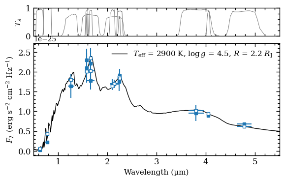
Plotting model spectrum and photometric fluxes
Finally, we will combine the model spectrum and the photometric fluxes in a plot with plot_spectrum. A list with Box objects is provided as an argument of boxes. These are interpreted accordingly by the
plot_spectrum function. Also a list with filter names can be provided as argument of filters to show the filter profiles. The ResidualsBox is provided as arguments of residuals. Finally, the optional argument of plot_kwargs contains a list with optional dictionaries to tune the
visualization of the plotted data. The number of items in the list of plot_kwargs should be equal to the number of items in the list of boxes. For the SynphotBox, we can set the item in plot_kwargs to None such that the marker design is based on the data from ObjectBox.
The blue squares are the photometric fluxes of PZ Tel B and the open squares are the synthetic photometry computed from the model spectrum. The residuals are shown relative to the uncertainties on the fluxes.
[17]:
fig = plot_spectrum(boxes=[modelbox, objectbox, synphot_box],
                    filters=objectbox.filters,
                    residuals=None,
                    plot_kwargs=[{'ls': '-', 'lw': 1., 'color': 'black'},
                                 {'Gemini/NICI.ED286': {'marker': 's', 'ms': 4., 'color': 'tab:blue', 'ls': 'none'},
                                  'Gemini/NIRI.H2S1v2-1-G0220': {'marker': 's', 'ms': 4., 'color': 'tab:blue', 'ls': 'none'},
                                  'Paranal/NACO.H': {'marker': 's', 'ms': 4., 'color': 'tab:blue', 'ls': 'none'},
                                  'Paranal/NACO.J': {'marker': 's', 'ms': 4., 'color': 'tab:blue', 'ls': 'none'},
                                  'Paranal/NACO.Ks': {'marker': 's', 'ms': 4., 'color': 'tab:blue', 'ls': 'none'},
                                  'Paranal/NACO.Lp': {'marker': 's', 'ms': 4., 'color': 'tab:blue', 'ls': 'none'},
                                  'Paranal/NACO.Mp': {'marker': 's', 'ms': 4., 'color': 'tab:blue', 'ls': 'none'},
                                  'Paranal/NACO.NB405': {'marker': 's', 'ms': 4., 'color': 'tab:blue', 'ls': 'none'},
                                  'Paranal/SPHERE.IRDIS_D_H23_2': {'marker': 's', 'ms': 4., 'color': 'tab:blue', 'ls': 'none'},
                                  'Paranal/SPHERE.IRDIS_D_H23_3': {'marker': 's', 'ms': 4., 'color': 'tab:blue', 'ls': 'none'},
                                  'Paranal/SPHERE.IRDIS_D_K12_1': {'marker': 's', 'ms': 4., 'color': 'tab:blue', 'ls': 'none'},
                                  'Paranal/SPHERE.IRDIS_D_K12_2': {'marker': 's', 'ms': 4., 'color': 'tab:blue', 'ls': 'none'},
                                  'Paranal/SPHERE.ZIMPOL_I_PRIM': {'marker': 's', 'ms': 4., 'color': 'tab:blue', 'ls': 'none'},
                                  'Paranal/SPHERE.ZIMPOL_R_PRIM': {'marker': 's', 'ms': 4., 'color': 'tab:blue', 'ls': 'none'}},
                                  None],
                    xlim=(0.5, 5.5),
                    legend={'loc': 'upper right', 'frameon': False, 'fontsize': 11.},
                    units=('um', 'erg s-1 cm-2 Hz-1'),
                    figsize=(5, 3),
                    output=None)
-------------
Plot spectrum
-------------

Boxes:
   - ModelBox
   - ObjectBox
   - SynphotBox

Object type: planet
Quantity: flux density
Units: ('um', 'erg s-1 cm-2 Hz-1')
Filter profiles: ['Gemini/NICI.ED286', 'Gemini/NIRI.H2S1v2-1-G0220', 'Paranal/NACO.H', 'Paranal/NACO.J', 'Paranal/NACO.Ks', 'Paranal/NACO.Lp', 'Paranal/NACO.Mp', 'Paranal/NACO.NB405', 'Paranal/SPHERE.IRDIS_D_H23_2', 'Paranal/SPHERE.IRDIS_D_H23_3', 'Paranal/SPHERE.IRDIS_D_K12_1', 'Paranal/SPHERE.IRDIS_D_K12_2', 'Paranal/SPHERE.ZIMPOL_I_PRIM', 'Paranal/SPHERE.ZIMPOL_R_PRIM']

Figure size: (5, 3)
Legend parameters: None
Include model name: False
The plot_spectrum function returned the Figure object of the plot. The functionalities of Matplotlib can be used for further customization of the plot. For example, the axes of the plot are stored at the axes attribute of Figure.
[18]:
fig.axes
[18]:
[<Axes: xlabel='Wavelength (µm)', ylabel='$F_\\lambda$ (erg s$^{-2}$ cm$^{-2}$ Hz$^{-1}$)'>,
 <Axes: ylabel='$T_\\lambda$'>]