Library with empirical spectra
In this tutorial, we will have a look at some brown dwarf spectra from the IRTF library. We will also calculate synthetic fluxes and combine the spectra and photometric fluxes in a plot.
Getting started
We start by importing species and initiating the database with the SpeciesInit class.
[1]:
from species import SpeciesInit
from species.data.database import Database
from species.read.read_spectrum import ReadSpectrum
from species.plot.plot_spectrum import plot_spectrum
[2]:
SpeciesInit()
=======
species
=======

Version: 0.10.3.dev11
Working folder: /Users/tomasstolker/applications/species/docs/tutorials

Creating species_config.ini... [DONE]
Creating species_database.hdf5... [DONE]
Creating data folder... [DONE]

Configuration settings:
   - Database: species_database.hdf5
   - Data folder: data
   - Magnitude of Vega: 0.03

Multiprocessing: mpi4py installed
Process number 1 out of 1...
[2]:
<species.core.species_init.SpeciesInit at 0x105bca3c0>
Adding a spectral library to the database
Next, we create an instance of Database, which is used for adding data to the database.
[3]:
database = Database()
We will now download and add the spectral library. For IRTF spectra, we can set the spectral types that we want to use. The parallax will be queried from SIMBAD and several VizieR catalogs. A warning will be printed in case no parallax can be retrieved and a NaN is stored. Therefore, computing an absolute, synthetic magnitude from these
spectra will not be possible.
[4]:
database.add_spectra(spec_library='irtf', sptypes=['L', 'T'])
Downloading data from 'https://home.strw.leidenuniv.nl/~stolker/species/parallax.dat' to file '/Users/tomasstolker/applications/species/docs/tutorials/data/parallax.dat'.
--------------------
Add spectral library
--------------------

Database tag: irtf
Spectral types: ['L', 'T']
100%|█████████████████████████████████████| 17.2k/17.2k [00:00<00:00, 60.9MB/s]
Downloading data from 'http://irtfweb.ifa.hawaii.edu/~spex/IRTF_Spectral_Library/Data/L_fits_091201.tar' to file '/Users/tomasstolker/applications/species/docs/tutorials/data/irtf/L_fits_091201.tar'.
100%|████████████████████████████████████████| 870k/870k [00:00<00:00, 545MB/s]
Downloading data from 'http://irtfweb.ifa.hawaii.edu/~spex/IRTF_Spectral_Library/Data/T_fits_091201.tar' to file '/Users/tomasstolker/applications/species/docs/tutorials/data/irtf/T_fits_091201.tar'.
100%|███████████████████████████████████████| 102k/102k [00:00<00:00, 72.2MB/s]
Unpacking IRTF Spectral Library...
 [DONE]

Adding spectra... [DONE]
WARNING: NoResultsWarning: The request executed correctly, but there was no data corresponding to these criteria in SIMBAD [astroquery.simbad.core]
Reading a spectral library
To read the spectra from the database, we first create an instance of ReadSpectrum. The full spectra are read if the argument of filter_name is set to None.
[5]:
read_spectrum = ReadSpectrum(spec_library='irtf', filter_name=None)
The spectra are extracted with the get_spectrum method and by providing a list of spectral types as argument for sptypes.
[6]:
specbox = read_spectrum.get_spectrum(sptypes=['L0', 'L1'])
The method returns a SpectrumBox with the requested data.
Opening a SpectrumBox
Let’s have a look at the attributes that are stored in the SpectrumBox by using the open_box method, which can be used on any of the Box objects. Among others, it contains the spectrum, the original names (from the IRTF library) and SIMBAD names, and the distances.
[7]:
specbox.open_box()
Opening SpectrumBox...
spectrum = None
wavelength = [array([0.8125008, 0.8125008, 0.8127338, ..., 4.126095 , 4.1269007,
       4.127706 ], shape=(6075,), dtype='>f4'), array([0.93558633, 0.93558633, 0.93585825, ..., 2.416591  , 2.4171278 ,
       2.417665  ], shape=(3383,), dtype='>f4'), array([0.8106775 , 0.8106775 , 0.81091094, ..., 4.113586  , 4.1143913 ,
       4.1151967 ], shape=(6059,), dtype='>f4')]
flux = [array([1.8895840e-14, 1.8895840e-14, 2.1758479e-14, ..., 3.7088523e-15,
       4.1113438e-15, 4.4284915e-15], shape=(6075,), dtype='>f4'), array([-1.0867816e-15, -1.0867816e-15,  2.5373139e-15, ...,
        2.0060095e-15,  2.1450817e-15,  2.2615936e-15],
      shape=(3383,), dtype='>f4'), array([3.8497135e-15, 3.8497135e-15, 2.5441878e-15, ..., 1.3200795e-15,
       1.2305833e-15, 1.0569799e-15], shape=(6059,), dtype='>f4')]
error = [array([2.5401353e-15, 2.5401353e-15, 2.8612678e-15, ..., 4.1515258e-16,
       4.3247181e-16, 4.4612945e-16], shape=(6075,), dtype='>f4'), array([2.2947999e-15, 2.2947999e-15, 1.3184451e-15, ..., 2.5160439e-16,
       1.7856300e-16, 9.8540571e-17], shape=(3383,), dtype='>f4'), array([1.9933140e-15, 1.9933140e-15, 2.2894352e-15, ..., 3.6852164e-16,
       3.4700822e-16, 3.5634480e-16], shape=(6059,), dtype='>f4')]
name = ['2MASS J07464256+2000321', '2MASS J02081833+2542533', '2MASS J14392836+1929149']
simbad = ['LSPM J0746+2000', '2MASS J02081833+2542533', '2MASS J14392836+1929149']
sptype = ['L0', 'L1', 'L1']
distance = None
spec_res = [nan, nan, nan]
spec_library = irtf
parallax = [(array([81.1]), array([0.9])), (np.float64(43.0992), np.float32(0.3249)), (array([69.6]), array([0.5]))]
Synthetic photometry
To calculate synthetic fluxes, we use again the ReadSpectrum class but we now also set the argument of filter_name to a filter as listed by the SVO Filter Profile Service. In this example, use an H-band filter from the MKO system.
[8]:
read_spectrum = ReadSpectrum(spec_library='irtf', filter_name='MKO/NSFCam.H')
The flux is now calculated with the get_flux method by again selecting the L0- and L1-type objects.
[9]:
photbox = read_spectrum.get_flux(sptypes=['L0', 'L1'])
Downloading data from 'https://archive.stsci.edu/hlsps/reference-atlases/cdbs/current_calspec/alpha_lyr_stis_011.fits' to file '/Users/tomasstolker/applications/species/docs/tutorials/data/alpha_lyr_stis_011.fits'.
100%|████████████████████████████████████████| 288k/288k [00:00<00:00, 294MB/s]
Adding spectrum: Vega
Reference: Bohlin et al. 2014, PASP, 126
URL: https://ui.adsabs.harvard.edu/abs/2014PASP..126..711B
Let’s have a look at the content of the returned PhotometryBox.
[10]:
photbox.open_box()
Opening PhotometryBox...
name = ['2MASS J07464256+2000321', '2MASS J02081833+2542533', '2MASS J14392836+1929149']
sptype = ['L0', 'L1', 'L1']
wavelength = [1.62982596 1.62982596 1.62982596]
flux = [[4.58844233e-14 8.29550575e-18]
 [6.09467685e-15 6.83240960e-18]
 [1.75018643e-14 5.23839232e-18]]
app_mag = None
abs_mag = None
filter_name = ['MKO/NSFCam.H' 'MKO/NSFCam.H' 'MKO/NSFCam.H']
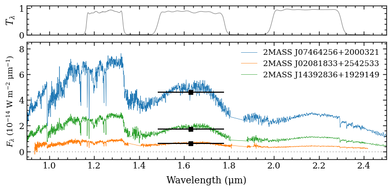
Plotting spectra and synthetic fluxes
Now that we have created a SpectrumBox and PhotometryBox, we pass them to the plot_spectrum function. The uncertainties on the spectral fluxes have been propagated into the synthetic photometric flux, but the uncertainties are smaller than the plotted markers. The horizontal “error bars” of the fluxes indicate the FWHM of the filter profile.
[11]:
fig = plot_spectrum(boxes=[specbox, photbox],
                    filters=['MKO/NSFCam.J', 'MKO/NSFCam.H', 'MKO/NSFCam.Ks'],
                    xlim=(0.9, 2.5),
                    ylim=(-6e-15, 8.5e-14),
                    offset=(-0.14, -0.03),
                    legend={'loc':'upper right', 'frameon': False, 'fontsize': 11.},
                    figsize=(7., 3.),
                    output=None)
-------------
Plot spectrum
-------------

Boxes:
   - SpectrumBox
   - PhotometryBox

Object type: planet
Quantity: flux density
Units: ('um', 'W m-2 um-1')
Filter profiles: ['MKO/NSFCam.J', 'MKO/NSFCam.H', 'MKO/NSFCam.Ks']

Figure size: (7.0, 3.0)
Legend parameters: None
Include model name: False
Font sizes: {'xlabel': 11.0, 'ylabel': 11.0, 'title': 13.0, 'legend': 9.0}
The plot_spectrum function returned the Figure object of the plot. The functionalities of Matplotlib can be used for further customization of the plot. For example, the axes of the plot are stored at the axes attribute of Figure.
[12]:
fig.axes
[12]:
[<Axes: xlabel='Wavelength (µm)', ylabel='$F_\\lambda$ (10$^{-14}$ W m$^{-2}$ µm$^{-1}$)'>,
 <Axes: ylabel='$T_\\lambda$'>]