Synthetic photometry

In this tutorial, we will obtain synthetic photometry in the F115W filter of JWST/NIRCam from an IRTF spectrum of Jupiter.

Getting started

We start by importing the required Python packages.

import urllib.request
import numpy as np
import matplotlib.pyplot as plt
import species

The species database that is specified in species_config.ini is initiated with the SpeciesInit class.

species.SpeciesInit()

Initiating species v0.1.4... [DONE]
Creating species_config.ini... [DONE]
Database: /Users/tomasstolker/applications/species/docs/tutorials/species_database.hdf5
Data folder: /Users/tomasstolker/applications/species/docs/tutorials/data
Working folder: /Users/tomasstolker/applications/species/docs/tutorials
Creating species_database.hdf5... [DONE]
Creating data folder... [DONE]

<species.core.setup.SpeciesInit at 0x12666a358>

Jupiter spectrum

The spectrum of Jupiter that is used as an example is now downloaded from the IRTF website.

urllib.request.urlretrieve('http://irtfweb.ifa.hawaii.edu/~spex/IRTF_Spectral_Library/Data/plnt_Jupiter.txt',
                           'data/plnt_Jupiter.txt')

('data/plnt_Jupiter.txt', <http.client.HTTPMessage at 0x1255d8d30>)

It contains the wavelength in \(\mu\)m, and the flux and uncertainty in W m\(^{-2}\) \(\mu\)m\(^-1\), which are also the units that species requires. We can read the data with loadtxt from numpy.

wavelength, flux, error = np.loadtxt('data/plnt_Jupiter.txt', unpack=True)

Let’s create a SpectrumBox with the data.

spec_box = species.create_box('spectrum',
                              spectrum='irtf',
                              wavelength=wavelength,
                              flux=flux,
                              error=error,
                              name='jupiter')

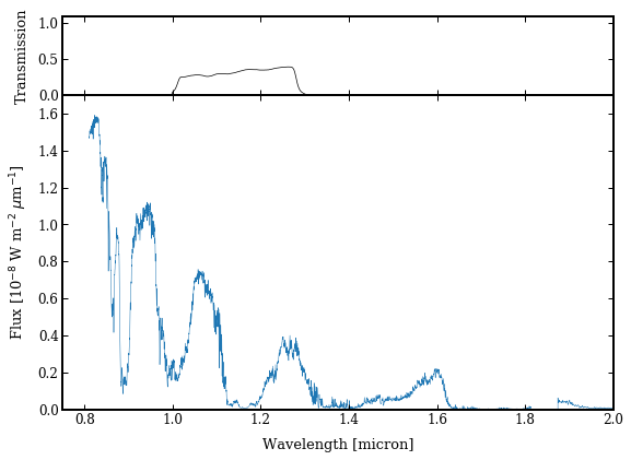
And pass the Box to the plot_spectrum function together with the filter name.

species.plot_spectrum(boxes=[spec_box, ],
                      filters=['JWST/NIRCam.F115W'],
                      xlim=(0.75, 2.),
                      ylim=(0., 1.7e-8),
                      offset=(-0.09, -0.06),
                      output='spectrum.png')

Adding filter: JWST/NIRCam.F115W... [DONE]
Plotting spectrum: spectrum.png... [DONE]

from IPython.display import Image
Image('spectrum.png')

Synthetic flux and magnitude

We use the SyntheticPhotometry class to calculate the flux and magnitude for the JWST/NIRCam.F115W filter.

synphot = species.SyntheticPhotometry('JWST/NIRCam.F115W')

The average flux in the JWST filter is calculated with the spectrum_to_flux function. The error on the synthetic flux is estimated with Monte Carlo sampling of the input spectrum.

jwst_flux = synphot.spectrum_to_flux(wavelength, flux, error=error)
print(f'Flux [W m-2 micron-1] = {jwst_flux[0]:.2e} +/- {jwst_flux[1]:.2e}')

Flux [W m-2 micron-1] = 2.64e-09 +/- 1.00e-13

Similarly, we can calculate the synthetic magnitude. Also the absolute magnitude can be calculated by providing the distance and uncertainty (set to None in the example). In species, the magnitude is defined relative to Vega, which is set to 0.03 mag. In this filter, Jupiter has a magnitude of 0.49 so the planet is similar in brightness to Vega.

jwst_mag, _ = synphot.spectrum_to_magnitude(wavelength, flux, error=error, distance=None)
print(f'Apparent magnitude [mag] = {jwst_mag[0]:.2f} +/- {jwst_mag[1]:.2e}')

Downloading Vega spectrum (270 kB)... [DONE]
Adding Vega spectrum... [DONE]
Apparent magnitude [mag] = 0.49 +/- 4.05e-05