Spectral library

In this tutorial, we will have a look at the L- and T-type spectra from the IRTF library. We will obtain synthetic photometry and combine these together with the spectra in a plot

Getting started

We start by importing species and initiating the database with the SpeciesInit class.

import species
species.SpeciesInit()

Initiating species v0.1.4... [DONE]
Creating species_config.ini... [DONE]
Database: /Users/tomasstolker/applications/species/docs/tutorials/species_database.hdf5
Data folder: /Users/tomasstolker/applications/species/docs/tutorials/data
Working folder: /Users/tomasstolker/applications/species/docs/tutorials
Creating species_database.hdf5... [DONE]
Creating data folder... [DONE]

<species.core.setup.SpeciesInit at 0x1044958d0>

Adding a spectral library to the database

A Database object is created, which is used for adding data to the database.

database = species.Database()

We now will now add the spectral library to the database. For IRTF spectra, we can set the spectral types that we want to download and add to the database. The parallax will be queried from SIMBAD and several VizieR catalogs. A warning will be printed in case no parallax can be retrieved in which case a NaN is stored as distance. Therefore, computing an absolute, synthetic magnitude from these spectra will not be possible.

database.add_spectrum(spec_library='irtf',
                      sptypes=['L', 'T'])

Downloading IRTF Spectral Library - L dwarfs (850 kB)... [DONE]
Downloading IRTF Spectral Library - T dwarfs (100 kB)... [DONE]
Unpacking IRTF Spectral Library... [DONE]
Adding IRTF Spectral Library... [DONE]

/Users/tomasstolker/.pyenv/versions/3.6.0/envs/general3.6/lib/python3.6/site-packages/astroquery/simbad/core.py:138: UserWarning: Warning: The script line number 3 raised an error (recorded in the `errors` attribute of the result table): 'DENIS-P 025503.3-470049.0': this identifier has an incorrect format for catalog:         DENIS : Deep Near-Infrared Survey
  (error.line, error.msg))
/Users/tomasstolker/applications/species/species/util/query_util.py:306: UserWarning: No parallax was found for DENIS-P 025503.3-470049.0 so storing a NaN value.
  warnings.warn(f'No parallax was found for {target} so storing a NaN value.')
/Users/tomasstolker/.pyenv/versions/3.6.0/envs/general3.6/lib/python3.6/site-packages/astroquery/simbad/core.py:138: UserWarning: Warning: The script line number 3 raised an error (recorded in the `errors` attribute of the result table): Identifier not found in the database : 2MASS J05591915-1404489
  (error.line, error.msg))
/Users/tomasstolker/applications/species/species/util/query_util.py:306: UserWarning: No parallax was found for 2MASS J05591915-1404489 so storing a NaN value.
  warnings.warn(f'No parallax was found for {target} so storing a NaN value.')

Reading a spectral library

We read the data of the spectral library from the database with the ReadSpectrum class. The full spectra are read when filter_name is set to None.

read_spectrum = species.ReadSpectrum(spec_library='irtf',
                                     filter_name=None)

The spectra are extracted with the get_spectrum function by setting the spectral types that we want to use.

specbox = read_spectrum.get_spectrum(sptypes=['L0', 'L1'])

Opening a SpectrumBox

Let’s have a look at the attributes that are stored in the SpectrumBox that was created by the get_spectrum function. Among others, it contains the spectrum, original names (from the IRTF library) and SIMBAD names, and distances.

specbox.open_box()

Opening SpectrumBox...
spectrum = None
wavelength = [array([0.8125008, 0.8125008, 0.8127338, ..., 4.126095 , 4.1269007,
       4.127706 ], dtype=float32)
 array([0.93558633, 0.93558633, 0.93585825, ..., 2.416591  , 2.4171278 ,
       2.417665  ], dtype=float32)
 array([0.8106775 , 0.8106775 , 0.81091094, ..., 4.113586  , 4.1143913 ,
       4.1151967 ], dtype=float32)]
flux = [array([1.8895840e-14, 1.8895840e-14, 2.1758479e-14, ..., 3.7088523e-15,
       4.1113438e-15, 4.4284915e-15], dtype=float32)
 array([-1.0867816e-15, -1.0867816e-15,  2.5373139e-15, ...,
        2.0060095e-15,  2.1450817e-15,  2.2615936e-15], dtype=float32)
 array([3.8497135e-15, 3.8497135e-15, 2.5441878e-15, ..., 1.3200795e-15,
       1.2305833e-15, 1.0569799e-15], dtype=float32)]
error = [array([2.5401353e-15, 2.5401353e-15, 2.8612678e-15, ..., 4.1515258e-16,
       4.3247181e-16, 4.4612945e-16], dtype=float32)
 array([2.2947999e-15, 2.2947999e-15, 1.3184451e-15, ..., 2.5160439e-16,
       1.7856300e-16, 9.8540571e-17], dtype=float32)
 array([1.9933140e-15, 1.9933140e-15, 2.2894352e-15, ..., 3.6852164e-16,
       3.4700822e-16, 3.5634480e-16], dtype=float32)]
name = ['2MASS J07464256+2000321' '2MASS J02081833+2542533'
 '2MASS J14392836+1929149']
simbad = ['LSPM J0746+2000' '2MASSW J0208183+254253' '2MASS J14392836+1929149']
sptype = ['L0' 'L1' 'L1']
distance = [[11.60092807  0.62084304]
 [23.65777607  0.35139512]
 [14.36781609  0.1032224 ]]
spec_library = irtf

Synthetic photometry

Similarly, we use the ReadSpectrum class to obtain synthetic photometry. In this case, we set the filter_name to the required tag from the SVO Filter Profile Service.

read_spectrum = species.ReadSpectrum(spec_library='irtf',
                                     filter_name='MKO/NSFCam.H')

Adding filter: MKO/NSFCam.H... [DONE]

We now use the get_flux function with again selecting the L0- and L1-type spectra from the database.

photbox = read_spectrum.get_flux(sptypes=['L0', 'L1'])

Plotting spectrum and synthetic fluxes

Now that we have created a SpectrumBox and PhotometryBox, we pass them to the plot_spectrum function.

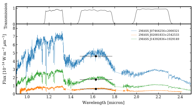
species.plot_spectrum(boxes=[specbox, photbox],
                      filters=['MKO/NSFCam.J', 'MKO/NSFCam.H', 'MKO/NSFCam.Ks'],
                      xlim=(0.9, 2.5),
                      ylim=(0., 8.5e-14),
                      offset=(-0.1, -0.045),
                      legend=(0.65, 0.75),
                      figsize=(8, 4),
                      output='spectrum.png')

Adding filter: MKO/NSFCam.J... [DONE]
Adding filter: MKO/NSFCam.Ks... [DONE]
Plotting spectrum: spectrum.png... [DONE]

Let’s have a look at the result! While the uncertainties are propagated with the synthetic photometry, the error bars are smaller than the plotted markers. The horizontal “error bars” of the fluxes indicate the FWHM of the filter profile.

from IPython.display import Image
Image('spectrum.png')