Fitting atmospheric spectra
In this tutorial, we will fit spectra and photometric fluxes of beta Pic b with the synthetic spectra from a radiative-convective equilibrium atmosphere model. Here we will use DRIFT-PHOENIX but there are also several other models supported by species.
Getting started
We start by setting the library path of MultiNest (see installation instructions), which is required for the Bayesian inference.
[1]:
import os
os.environ['DYLD_LIBRARY_PATH'] = '/Users/tomasstolker/applications/MultiNest/lib'
We also need to import pooch and the species toolkit.
[2]:
import pooch
from species import SpeciesInit
from species.data.database import Database
from species.fit.fit_model import FitModel
from species.read.read_model import ReadModel
from species.plot.plot_mcmc import plot_posterior
from species.plot.plot_spectrum import plot_spectrum
from species.util.box_util import update_objectbox
from species.util.fit_util import get_residuals, multi_photometry
We initiate species by running the SpeciesInit class. By doing so, both the configuration file and the HDF5 database are created in the working folder.
[3]:
SpeciesInit()
=======
species
=======

Version: 0.10.0
Working folder: /Users/tomasstolker/applications/species/docs/tutorials

Creating species_config.ini... [DONE]
Creating species_database.hdf5... [DONE]
Creating data folder... [DONE]

Configuration settings:
   - Database: species_database.hdf5
   - Data folder: data
   - Magnitude of Vega: 0.03

Multiprocessing: mpi4py installed
Process number 1 out of 1...
[3]:
<species.core.species_init.SpeciesInit at 0x10429d400>
Let’s now download the GRAVITY \(K\) band spectrum of beta Pic b that was published by Gravity Collaboration et al. 2020 and we will also make use of the GPI \(YJH\) band spectra from Chilcote et al. 2017.
[4]:
data_urls = ['https://home.strw.leidenuniv.nl/~stolker/species/spectra/BetaPictorisb_2018-09-22.fits',
             'https://home.strw.leidenuniv.nl/~stolker/species/spectra/betapicb_gpi_y.dat',
             'https://home.strw.leidenuniv.nl/~stolker/species/spectra/betapicb_gpi_j.dat',
             'https://home.strw.leidenuniv.nl/~stolker/species/spectra/betapicb_gpi_h.dat']
[5]:
for url in data_urls:
    pooch.retrieve(
        url=url,
        known_hash=None,
        fname=url.split('/')[-1],
        path='./',
        progressbar=True,
    )
Downloading data from 'https://home.strw.leidenuniv.nl/~stolker/species/spectra/BetaPictorisb_2018-09-22.fits' to file '/Users/tomasstolker/applications/species/docs/tutorials/BetaPictorisb_2018-09-22.fits'.
100%|███████████████████████████████████████| 913k/913k [00:00<00:00, 1.94GB/s]
SHA256 hash of downloaded file: 4b4507e4af6cec5711d2110974061584b8d23cc108daae7fa3be8c27d866847c
Use this value as the 'known_hash' argument of 'pooch.retrieve' to ensure that the file hasn't changed if it is downloaded again in the future.
Downloading data from 'https://home.strw.leidenuniv.nl/~stolker/species/spectra/betapicb_gpi_y.dat' to file '/Users/tomasstolker/applications/species/docs/tutorials/betapicb_gpi_y.dat'.
100%|█████████████████████████████████████| 1.50k/1.50k [00:00<00:00, 5.92MB/s]
SHA256 hash of downloaded file: 93471c556d69a25f2fe9b5ff1ed9fe7e442ec6ad35983c17663be79e35d793c6
Use this value as the 'known_hash' argument of 'pooch.retrieve' to ensure that the file hasn't changed if it is downloaded again in the future.
Downloading data from 'https://home.strw.leidenuniv.nl/~stolker/species/spectra/betapicb_gpi_j.dat' to file '/Users/tomasstolker/applications/species/docs/tutorials/betapicb_gpi_j.dat'.
100%|█████████████████████████████████████| 1.65k/1.65k [00:00<00:00, 7.65MB/s]
SHA256 hash of downloaded file: 8c064e4cc652d360d043d6c4315ec2f6a8f4cf652869895294e8a6d08b8891be
Use this value as the 'known_hash' argument of 'pooch.retrieve' to ensure that the file hasn't changed if it is downloaded again in the future.
Downloading data from 'https://home.strw.leidenuniv.nl/~stolker/species/spectra/betapicb_gpi_h.dat' to file '/Users/tomasstolker/applications/species/docs/tutorials/betapicb_gpi_h.dat'.
100%|█████████████████████████████████████| 1.75k/1.75k [00:00<00:00, 6.66MB/s]
SHA256 hash of downloaded file: 5a04196497d22ea038729207558f4e432ebc7408d0da3ada53fa070e9cc41332
Use this value as the 'known_hash' argument of 'pooch.retrieve' to ensure that the file hasn't changed if it is downloaded again in the future.
Adding model spectra to the database
Data will be added to the database by first creating an instance of Database.
[6]:
database = Database()
The Database object has a number of methods to read and write data. For adding model spectra, we use the add_model method which will download the grid of DRIFT-PHOENIX spectra to the data_folder (see configuration file) except if the data was already present. After downloading, it will import
the spectra into the database. We will only require a limited range of \(T_\mathrm{eff}\) since we know the approximate temperature of beta Pic b.
[7]:
database.add_model(model='drift-phoenix', teff_range=(1500., 2000.))
Downloading data from 'https://home.strw.leidenuniv.nl/~stolker/species/drift-phoenix.tgz' to file '/Users/tomasstolker/applications/species/docs/tutorials/data/drift-phoenix.tgz'.
-------------------------
Add grid of model spectra
-------------------------

Database tag: drift-phoenix
Model name: DRIFT-PHOENIX
100%|████████████████████████████████████████| 113M/113M [00:00<00:00, 224GB/s]
Unpacking 140/496 model spectra from DRIFT-PHOENIX (109 MB)... [DONE]

Please cite Helling et al. (2008) when using DRIFT-PHOENIX in a publication
Reference URL: https://ui.adsabs.harvard.edu/abs/2008ApJ...675L.105H

Wavelength range (um) = 0.1 - 500
Sampling (lambda/d_lambda) = 2000
Teff range (K) = 1500.0 - 2000.0

Adding DRIFT-PHOENIX model spectra... data/drift-phoenix/drift-phoenix_teff_2000_logg_5.5_feh_0.3_spec.npy

Grid points stored in the database:
   - Teff = [1500. 1600. 1700. 1800. 1900. 2000.]
   - log(g) = [3.  3.5 4.  4.5 5.  5.5]
   - [Fe/H] = [-0.6 -0.3 -0.   0.3]

Number of grid points per parameter:
   - teff: 6
   - logg: 6
   - feh: 4

Fix missing grid points with a linear interpolation:
   - teff = 1600.0, logg = 3.0, feh = 0.3
   - teff = 1600.0, logg = 5.5, feh = 0.3
   - teff = 1900.0, logg = 4.5, feh = 0.3
   - teff = 1900.0, logg = 5.5, feh = 0.3

Number of stored grid points: 144
Number of interpolated grid points: 4
Number of missing grid points: 0
/Users/tomasstolker/applications/species/species/util/data_util.py:413: RuntimeWarning: divide by zero encountered in log10
  flux = np.log10(flux)
Adding photometry and spectra
We will also add photometric data of beta Pic b that have been adopted in species from various references. To get an overview of all photometric data that were stored in the database, we can use the list_companions method of the
Database object (i.e. database.list_companions() in this case).
To add the photometric data and parallax of beta Pic b to the database, we use the add_companion method, which will also convert the magnitudes into fluxes with a flux-calibrated spectrum of Vega and the filter profiles (downloaded from the SVO Filter Profile Service). It is also possible to manually add photometric data with the
app_mag and flux_density arguments of add_object.
[8]:
database.add_companion(name='beta Pic b')
---------------------
Get companion spectra
---------------------

Getting GPI_YJHK spectrum of beta Pic b...
Downloading data from 'https://home.strw.leidenuniv.nl/~stolker/species/spectra/betapicb_gpi_yjhk.dat' to file '/Users/tomasstolker/applications/species/docs/tutorials/data/companion_data/betapicb_gpi_yjhk.dat'.
100%|█████████████████████████████████████| 8.50k/8.50k [00:00<00:00, 37.1MB/s]
SHA256 hash of downloaded file: 33e8d3ee32aa661f97624eda64e4a7f67dac2a7f22a072136a8414713379ef50
Use this value as the 'known_hash' argument of 'pooch.retrieve' to ensure that the file hasn't changed if it is downloaded again in the future.
 [DONE]
Please cite Chilcote et al. 2017, AJ, 153, 182 when making use of this spectrum in a publication
Getting GRAVITY spectrum of beta Pic b...
Downloading data from 'https://home.strw.leidenuniv.nl/~stolker/species/spectra/BetaPictorisb_2018-09-22.fits' to file '/Users/tomasstolker/applications/species/docs/tutorials/data/companion_data/BetaPictorisb_2018-09-22.fits'.
100%|███████████████████████████████████████| 913k/913k [00:00<00:00, 1.46GB/s]
SHA256 hash of downloaded file: 4b4507e4af6cec5711d2110974061584b8d23cc108daae7fa3be8c27d866847c
Use this value as the 'known_hash' argument of 'pooch.retrieve' to ensure that the file hasn't changed if it is downloaded again in the future.
Downloading data from 'https://xwcl.science/magao/visao/VisAO_Ys_filter_curve.dat' to file '/Users/tomasstolker/applications/species/docs/tutorials/data/VisAO_Ys_filter_curve.dat'.
 [DONE]
Please cite Gravity Collaboration et al. 2020, A&A, 633, 110 when making use of this spectrum in a publication

----------
Add object
----------

Object name: beta Pic b
Units: None
Deredden: None
SHA256 hash of downloaded file: 4d523a06d8daae91f91d98f4ee8dacbfef7d17c6161a4c217dd56cd6006b9d56
Use this value as the 'known_hash' argument of 'pooch.retrieve' to ensure that the file hasn't changed if it is downloaded again in the future.
Downloading data from 'https://archive.stsci.edu/hlsps/reference-atlases/cdbs/current_calspec/alpha_lyr_stis_011.fits' to file '/Users/tomasstolker/applications/species/docs/tutorials/data/alpha_lyr_stis_011.fits'.
100%|████████████████████████████████████████| 288k/288k [00:00<00:00, 524MB/s]
Adding spectrum: Vega
Reference: Bohlin et al. 2014, PASP, 126
URL: https://ui.adsabs.harvard.edu/abs/2014PASP..126..711B/abstract
Parallax (mas) = 50.93 +/- 0.15

Magnitudes:
   - Magellan/VisAO.Ys:
      - Mean wavelength (um) = 9.8268e-01
      - Apparent magnitude = 15.53 +/- 0.34
      - Flux (W m-2 um-1) = 4.21e-15 +/- 1.34e-15
   - Paranal/NACO.J:
      - Mean wavelength (um) = 1.2651e+00
      - Apparent magnitude = 14.11 +/- 0.21
      - Flux (W m-2 um-1) = 6.78e-15 +/- 1.32e-15
   - Gemini/NICI.ED286:
      - Mean wavelength (um) = 1.5842e+00
      - Apparent magnitude = 13.18 +/- 0.15
      - Flux (W m-2 um-1) = 6.88e-15 +/- 9.54e-16
   - Paranal/NACO.H:
      - Mean wavelength (um) = 1.6588e+00
      - Apparent magnitude = 13.32 +/- 0.14
      - Flux (W m-2 um-1) = 5.39e-15 +/- 6.96e-16
   - Paranal/NACO.Ks:
      - Mean wavelength (um) = 2.1450e+00
      - Apparent magnitude = 12.64 +/- 0.11
      - Flux (W m-2 um-1) = 3.97e-15 +/- 4.03e-16
   - Paranal/NACO.NB374:
      - Mean wavelength (um) = 3.7448e+00
      - Apparent magnitude = 11.25 +/- 0.23
      - Flux (W m-2 um-1) = 1.66e-15 +/- 3.54e-16
   - Paranal/NACO.Lp:
      - Mean wavelength (um) = 3.8050e+00
      - Apparent magnitude = 11.30 +/- 0.06
      - Flux (W m-2 um-1) = 1.56e-15 +/- 8.61e-17
   - Paranal/NACO.NB405:
      - Mean wavelength (um) = 4.0559e+00
      - Apparent magnitude = 10.98 +/- 0.05
      - Flux (W m-2 um-1) = 1.58e-15 +/- 7.27e-17
   - Paranal/NACO.Mp:
      - Mean wavelength (um) = 4.7810e+00
      - Apparent magnitude = 11.10 +/- 0.12
      - Flux (W m-2 um-1) = 7.70e-16 +/- 8.52e-17

Spectra:
   - Spectrum:
      - Database tag: GPI_YJHK
      - Filename: data/companion_data/betapicb_gpi_yjhk.dat
      - Data shape: (152, 3)
      - Wavelength range (um): 0.98 - 2.37
      - Mean flux (W m-2 um-1): 5.40e-15
      - Mean error (W m-2 um-1): 6.44e-16
   - GRAVITY spectrum:
      - Object: Unknown
      - Database tag: GRAVITY
      - Filename: data/companion_data/BetaPictorisb_2018-09-22.fits
      - Data shape: (237, 3)
      - Wavelength range (um): 1.97 - 2.49
      - Mean flux (W m-2 um-1): 4.65e-15
      - Mean error (W m-2 um-1): 1.00e-16
   - GRAVITY covariance matrix:
      - Object: Unknown
      - Database tag: GRAVITY
      - Filename: data/companion_data/BetaPictorisb_2018-09-22.fits
      - Data shape: (237, 237)
   - Instrument resolution:
      - GPI_YJHK: 40.0
      - GRAVITY: 500.0
/Users/tomasstolker/applications/species/species/data/database.py:1521: UserWarning: Found 33 fluxes with NaN in the data of GPI_YJHK. Removing the spectral fluxes that contain a NaN.
  warnings.warn(
Next, we will add the spectra with the add_object method. Make sure to use the same database name as argument of object_name (i.e. beta Pic b in this case) such that the spectra are added to the object name for which previously photometric data had been stored with
add_companion.
The argument of spectrum is a dictionary with the names of the spectra as key and a tuple with three elements as value. The first element is a text or FITS file with the spectrum, the second element is the optional covariance matrix, and the third value is the mandatory spectral resolution. The latter is used to smooth the model spectra to the instrument resolution.
For this example, we have adopted the VLTI/GRAVITY \(K\) band spectrum from Gravity Collaboration et al. 2020 and the Gemini/GPI \(YJH\) band spectra from Chilcote et al. 2017. Data that have been stored in the FITS format by the ExoGRAVITY collaboration is automatically recognized so the same FITS filename can be provided as first and second element in the dictionary.
[9]:
database.add_object('beta Pic b',
                    parallax=None,
                    app_mag=None,
                    flux_density=None,
                    spectrum={'GRAVITY': ('BetaPictorisb_2018-09-22.fits', 'BetaPictorisb_2018-09-22.fits', 500.),
                              'GPI_Y': ('betapicb_gpi_y.dat', None, 40.),
                              'GPI_J': ('betapicb_gpi_j.dat', None, 40.),
                              'GPI_H': ('betapicb_gpi_h.dat', None, 40.)},
                    deredden=None)
----------
Add object
----------

Object name: beta Pic b
Units: None
Deredden: None

Spectra:
   - GRAVITY spectrum:
      - Object: Unknown
      - Database tag: GRAVITY
      - Filename: BetaPictorisb_2018-09-22.fits
      - Data shape: (237, 3)
      - Wavelength range (um): 1.97 - 2.49
      - Mean flux (W m-2 um-1): 4.65e-15
      - Mean error (W m-2 um-1): 1.00e-16
   - Spectrum:
      - Database tag: GPI_Y
      - Filename: betapicb_gpi_y.dat
      - Data shape: (29, 3)
      - Wavelength range (um): 0.98 - 1.13
      - Mean flux (W m-2 um-1): 5.40e-15
      - Mean error (W m-2 um-1): 1.87e-15
   - Spectrum:
      - Database tag: GPI_J
      - Filename: betapicb_gpi_j.dat
      - Data shape: (32, 3)
      - Wavelength range (um): 1.13 - 1.34
      - Mean flux (W m-2 um-1): 6.84e-15
      - Mean error (W m-2 um-1): 4.79e-16
   - Spectrum:
      - Database tag: GPI_H
      - Filename: betapicb_gpi_h.dat
      - Data shape: (34, 3)
      - Wavelength range (um): 1.51 - 1.79
      - Mean flux (W m-2 um-1): 5.63e-15
      - Mean error (W m-2 um-1): 3.86e-16
   - GRAVITY covariance matrix:
      - Object: Unknown
      - Database tag: GRAVITY
      - Filename: BetaPictorisb_2018-09-22.fits
      - Data shape: (237, 237)
   - Instrument resolution:
      - GRAVITY: 500.0
      - GPI_Y: 40.0
      - GPI_J: 40.0
      - GPI_H: 40.0
The use of add_object is incremental so when rerunning the method it will add new data in case a filter or spectrum name hadn’t been used before, or it will overwrite existing data in case a filter or spectrum name does already exist. To remove existing data of an object, it is easiest to remove the group of data entirely from the database with the
delete_data method of Database (e.g. delete_data('objects/beta Pic b') and rerun add_companion and/or
add_object afterwards.
Bayesian inference with nested sampling
To fit the data with the grid of model spectra (i.e. grid retrieval), we start by creating an instance of FitModel, which requires the database tag of the object (beta Pic b) and the atmosphere model (drift-phoenix).
The dictionary of the bounds parameter contains the prior boundaries for the various parameters. By default, the parameters of the atmosphere model are set to the full range of the available spectra (e.g. \(\log(g)\) and \(\mathrm{[Fe/H]}\) in the example below).
In addition to the parameters of the atmosphere model, several optional parameters can be fitted, for example to account for calibration systematics, extinction, and excess emission from a disk. More details on the various parameters can be found in the API documentation of FitModel. As example, we fit a scaling parameter for the GPI \(H\) band spectrum.
The arguments of inc_phot and inc_spec are either a boolean or a list of photometry and spectra that were previously stored in the database for the object beta Pic b. We will use all the spectra but only the photometric data in the \(L\) and \(M\) bands.
To account for correlated noise, it is possible to apply the approach from Wang et al. (2020) to estimate the covariances by using a Gaussian process. This will add two additional parameters per spectrum (correlation length and amplitude) but is not mandatory. For the example, we only select the GPI \(H\) band spectrum, to limit the computation time.
For simplicity we create a list with the 4 filter names that we want to use.
[10]:
inc_phot = ['Paranal/NACO.Lp', 'Paranal/NACO.NB374', 'Paranal/NACO.NB405', 'Paranal/NACO.Mp']
We now create the instance of FitModel. By doing so, the grid of model spectra will be interpolated to the wavelengths of the data.
[11]:
fit = FitModel(object_name='beta Pic b',
               model='drift-phoenix',
               bounds={'teff': (1500., 2000.),
                       'radius': (0.5, 2.),
                       'scaling_GPI_H': (0.5, 1.5)},
               inc_phot=inc_phot,
               inc_spec=True,
               fit_corr=None,
               apply_weights=False,
               normal_prior={'mass': (9., 1.6)})
-----------------
Fit model spectra
-----------------

Object name: beta Pic b
Model tag: drift-phoenix
Binary star: False
Blackbody components: 0
Teff interpolation range: (1500.0, 2000.0)

Interpolating Paranal/NACO.Lp... [DONE]
Interpolating Paranal/NACO.NB374... [DONE]
Interpolating Paranal/NACO.NB405... [DONE]
Interpolating Paranal/NACO.Mp... [DONE]
Interpolating GPI_H... [DONE]
Interpolating GPI_J... [DONE]
Interpolating GPI_Y... [DONE]
Interpolating GPI_YJHK... [DONE]
Interpolating GRAVITY... [DONE]

Fitting 6 parameters:
   - teff
   - logg
   - feh
   - radius
   - parallax
   - scaling_GPI_H

Uniform priors (min, max):
   - teff = (1500.0, 2000.0)
   - radius = (0.5, 2.0)
   - scaling_GPI_H = (0.5, 1.5)
   - logg = (np.float64(3.0), np.float64(5.5))
   - feh = (np.float64(-0.6), np.float64(0.3))

Normal priors (mean, sigma):
   - mass = 9.00 +/- 1.60
   - parallax = 50.93 +/- 0.15

Weights for the log-likelihood function:
   - GPI_H = 1.00
   - GPI_J = 1.00
   - GPI_Y = 1.00
   - GPI_YJHK = 1.00
   - GRAVITY = 1.00
   - Paranal/NACO.Lp = 1.00
   - Paranal/NACO.NB374 = 1.00
   - Paranal/NACO.NB405 = 1.00
   - Paranal/NACO.Mp = 1.00
We are now ready to sample the posterior distribution by either using MultiNest, UltraNest, or Dynesty with the run_multinest,
run_ultranest, and run_dynesty methods of FitModel. Both are nested sampling algorithms which are powerful in sampling multi-modal distributions and will estimate the marginalized likelihood (i.e. model evidence), which enables pair-wise model comparison through the Bayes
factor.
In this example, we will use the run_multinest method. We specify the database tag were the posterior samples will be stored, the number of live points, the output folder where MultiNest will write its data, and we use the mass of beta Pic b from Gravity Collaboration et al. 2020 as Gaussian prior on
\(\log(g)\).
To speed up the computation, it is possible to run the nested sampling in parallel (e.g. with mpirun) to benefit from the multiprocessing support by MultiNest, UltraNest, and Dynesty. In that case it is important that any functions of species that will write to the Database will be commented out since simultaneous writing to the HDF5 database by different processes is not possible.
It is therefore recommended to first add all the required data to the database and then only run SpeciesInit, FitModel, and the sampler (run_multinest,
run_ultranest, run_dynesty) in parallel with MPI.
[12]:
fit.run_multinest(tag='betapic',
                  n_live_points=500,
                  resume=False,
                  output='multinest/',
                  kwargs_multinest=None)
------------------------------
Nested sampling with MultiNest
------------------------------

Database tag: betapic
Number of live points: 500
Resume previous fit: False
Output folder: multinest/

 *****************************************************
 MultiNest v3.10
 Copyright Farhan Feroz & Mike Hobson
 Release Jul 2015

 no. of live points =  500
 dimensionality =    6
 *****************************************************
 ln(ev)=   16470.539236937235      +/-  0.19128365808260553
 Total Likelihood Evaluations:        44271
 Sampling finished. Exiting MultiNest

log-evidence = 16470.54 +/- 0.19
log-evidence (importance sampling) = 16469.09 +/- 0.16

Sample with the maximum likelihood:
   - Log-likelihood = 16491.51
   - teff = 1710.56
   - logg = 3.84
   - feh = 0.12
   - radius = 1.49
   - parallax = 50.92
   - scaling_GPI_H = 1.10

---------------------
Add posterior samples
---------------------

Database tag: betapic
Sampler: multinest
Samples shape: (2808, 6)
ln(Z) = 16470.54 +/- 0.19
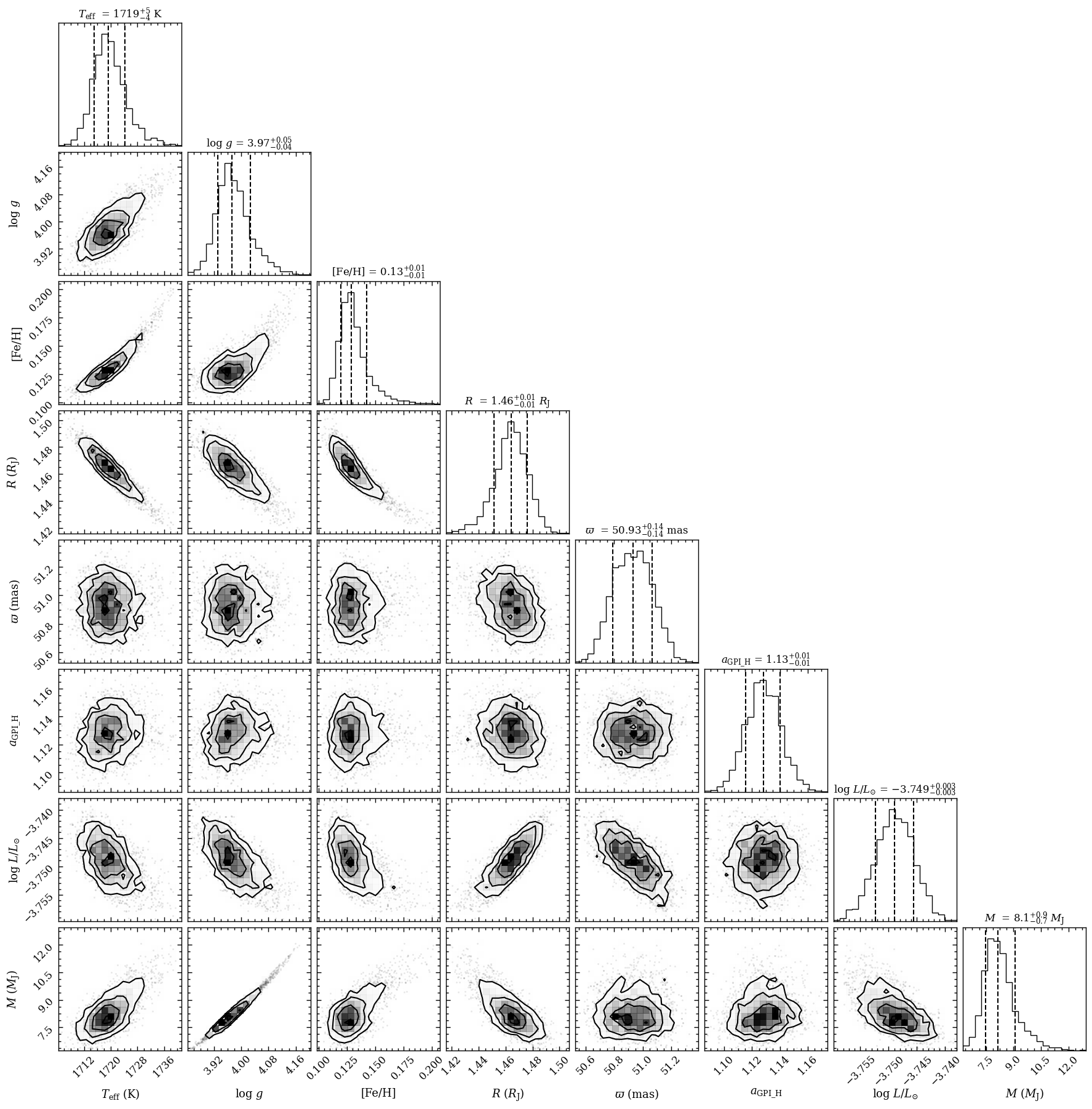
Plotting the posterior samples
The samples from the parameter estimation have been stored in the database. We can now run the plot_posterior function to plot the 1D and 2D projections of the posterior distributions by making use of corner.py. Here we specify the database tag with the results from run_multinest and we also include the derived posterior for the bolometric luminosity and mass.
[12]:
fig = plot_posterior(tag='betapic',
                     offset=(-0.3 , -0.3),
                     title_fmt=['.0f', '.2f', '.2f', '.2f', '.2f', '.2f', '.3f', '.1f'],
                     inc_luminosity=True,
                     inc_mass=True,
                     output=None)
Median sample:
   - teff = 1.72e+03
   - logg = 3.97e+00
   - feh = 1.29e-01
   - radius = 1.46e+00
   - parallax = 5.09e+01
   - scaling_GPI_H = 1.13e+00
Maximum posterior sample:
   - teff = 1.72e+03
   - logg = 3.97e+00
   - feh = 1.25e-01
   - radius = 1.47e+00
   - parallax = 5.07e+01
   - scaling_GPI_H = 1.12e+00
Plotting the posterior...
[DONE]
The plot_posterior function returned the Figure object of the plot. The functionalities of Matplotlib can be used for further customization of the plot. For example, the axes of the plot are stored at the axes attribute of Figure.
Extracting boxes with results
We will now extract Box objects with the results. These will be combined in a plot at the end of the tutorial. We start by selecting 30 random samples from the posterior and use these parameters to interpolate the DRIFT-PHOENIX grid. To do so, we use the get_mcmc_spectra method of the Database. We will smooth the spectra to a resolution of \(R=500\) to match with the resolution of the GRAVITY spectrum.
[12]:
samples = database.get_mcmc_spectra(tag='betapic',
                                    random=30,
                                    wavel_range=None,
                                    spec_res=500.)
The function returned a list with 30 ModelBox objects. Let’s have a look at the content of the first box by running the open_box method. This method can be used for all boxes to easily inspect the attributes of a Box object.
[13]:
samples[0].open_box()
Opening ModelBox...
model = drift-phoenix
type = None
wavelength = [ 0.1         0.10002476  0.10004953 ... 49.97524871 49.98762282
 50.        ]
flux = [1.65779100e-69 1.52878878e-69 1.36270592e-69 ... 2.09975833e-19
 2.09742153e-19 2.09579789e-19]
parameters = {'teff': 1717.4046446676018, 'logg': 3.9488578965346766, 'feh': 0.11823452057440464, 'radius': 1.476022338096074, 'parallax': 50.836805513590505, 'luminosity': 0.00018031877886305145, 'mass': 7.813186831275232}
quantity = flux
contribution = None
bol_flux = None
Instead of using the plotting functionalities of species, the attributes from a Box can also be directly extracted for further processing. For example, to print the wavelengths of the first ModelBox that was returned by
get_mcmc_spectra:
[14]:
print(samples[0].wavelength)
[ 0.1         0.10002476  0.10004953 ... 49.97524871 49.98762282
 50.        ]
Next, we get the median parameter values with the get_median_sample method of the Database and adopt these as best-fit parameters. Similarly, the get_probable_sample method can be used for extracting the sample with the maximum likelihood.
[15]:
best = database.get_median_sample(tag='betapic')
The best-fit model spectrum is now extracted from the DRIFT-PHOENIX grid by using the functionalities of the ReadModel class.
[16]:
read_model = ReadModel(model='drift-phoenix', wavel_range=None)
The grid is interpolated at the best-fit parameters with get_model. The argument of model_param contains the parameter dictionary that was returned by get_median_sample. The spectrum will be smoothed to a resolution of \(R=500\). To extract the spectrum without
smoothing at the resolution as stored in the database is achieved by setting spec_res=None and smooth=False.
[17]:
modelbox = read_model.get_model(model_param=best,
                                spec_res=500.,
                                smooth=True)
/Users/tomasstolker/applications/species/species/read/read_model.py:789: UserWarning: The 'scaling_GPI_H' parameter is not required by 'drift-phoenix' so the parameter will be ignored. The mandatory parameters are ['teff', 'logg', 'feh'].
  warnings.warn(
Some warnings are printed because the model_param dictionary contained calibration parameters (that were fitted), but these are not required when reading a model spectrum.
We will also extract all spectra and photometric fluxes of beta Pic b with the get_object method which will return the output in an ObjectBox.
[18]:
objectbox = database.get_object(object_name='beta Pic b',
                                inc_phot=True,
                                inc_spec=True)
Getting object: beta Pic b... [DONE]
We then run the ObjectBox through the update_objectbox function with the best-fit parameters. This function applies the flux scaling and could also inflate the errors in case the model_param dictionary contains error inflation parameters.
[19]:
objectbox = update_objectbox(objectbox=objectbox, model_param=best)
Scaling the flux of GPI_H by: 1.13... [DONE]
Next, we calculate the residuals of the best-fit model with get_residuals. This function will interpolate the grid at the specified parameters, calculate synthetic photometry for the filters that are provided as argument of inc_phot, and smooth and resample the spectra to the resolution and wavelengths of the spectra that are provided as argument of inc_spec (all spectra of the
ObjectBox in this case). The returned residuals will be stored in a ResidualsBox.
[20]:
residuals = get_residuals(datatype='model',
                          spectrum='drift-phoenix',
                          parameters=best,
                          objectbox=objectbox,
                          inc_phot=inc_phot,
                          inc_spec=True)
Calculating synthetic photometry... [DONE]
Calculating residuals... [DONE]
Residuals (sigma):
   - Paranal/NACO.Lp: -5.22
   - Paranal/NACO.NB374: -1.24
   - Paranal/NACO.NB405: -1.20
   - Paranal/NACO.Mp: -1.01
   - GPI_H: min: -1.18, max: 2.08
   - GPI_J: min: -1.89, max: 3.99
   - GPI_Y: min: -1.35, max: 1.37
   - GRAVITY: min: -5.74, max: 5.13
Reduced chi2 = 2.85
Number of degrees of freedom = 330
Finally, we compute synthetic photometry from the best-fit model spectrum with the multi_photometry function. Since we will plot all available photometric data of the ObjectBox, we will calculate synthetic photometry for all the names of the filters attribute of the
ObjectBox.
[21]:
synphot = multi_photometry(datatype='model',
                           spectrum='drift-phoenix',
                           filters=objectbox.filters,
                           parameters=best)
Calculating synthetic photometry... [DONE]
Let’s have a look inside the SynphotBox.
[22]:
synphot.open_box()
Opening SynphotBox...
name = synphot
wavelength = {'Gemini/NICI.ED286': 1.5841803431418238, 'Magellan/VisAO.Ys': 0.9826820974261752, 'Paranal/NACO.H': 1.6588090664617747, 'Paranal/NACO.J': 1.265099894847529, 'Paranal/NACO.Ks': 2.144954491491888, 'Paranal/NACO.Lp': 3.8050282724280526, 'Paranal/NACO.Mp': 4.780970919324577, 'Paranal/NACO.NB374': 3.744805012092439, 'Paranal/NACO.NB405': 4.055862923806052}
flux = {'Gemini/NICI.ED286': 6.314574982500849e-15, 'Magellan/VisAO.Ys': 3.2578689248914693e-15, 'Paranal/NACO.H': 6.0246080083049646e-15, 'Paranal/NACO.J': 6.376391872256607e-15, 'Paranal/NACO.Ks': 4.983988754633537e-15, 'Paranal/NACO.Lp': 2.005966104130527e-15, 'Paranal/NACO.Mp': 8.554095320982633e-16, 'Paranal/NACO.NB374': 2.096452509187913e-15, 'Paranal/NACO.NB405': 1.6647056387323192e-15}
app_mag = {'Gemini/NICI.ED286': (13.273857253310725, None), 'Magellan/VisAO.Ys': (15.809512953734055, None), 'Paranal/NACO.H': (13.198296363961237, None), 'Paranal/NACO.J': (14.177326064050416, None), 'Paranal/NACO.Ks': (12.393618660175498, None), 'Paranal/NACO.Lp': (11.02464211263265, None), 'Paranal/NACO.Mp': (10.985177418908139, None), 'Paranal/NACO.NB374': (10.995440399070313, None), 'Paranal/NACO.NB405': (10.921465476087254, None)}
abs_mag = {'Gemini/NICI.ED286': (11.808675674225412, None), 'Magellan/VisAO.Ys': (14.344331374648743, None), 'Paranal/NACO.H': (11.733114784875925, None), 'Paranal/NACO.J': (12.712144484965103, None), 'Paranal/NACO.Ks': (10.928437081090186, None), 'Paranal/NACO.Lp': (9.559460533547337, None), 'Paranal/NACO.Mp': (9.519995839822826, None), 'Paranal/NACO.NB374': (9.530258819985, None), 'Paranal/NACO.NB405': (9.456283897001942, None)}
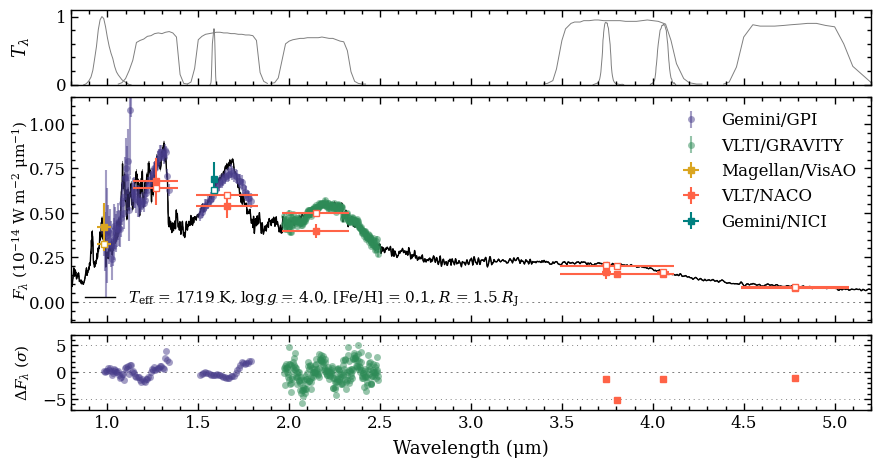
Plotting the spectral energy distribution
Now that we have gathered all the Box objects with the results, we can pass them as list to the boxes parameter of the plot_spectrum function. The ResidualsBox is separately provided as argument of residuals. We also include a list of filter names for which the transmission profiles
will be plotted. The arguments of residuals and filters can also be set to None to not include these data in the plot.
The somewhat complex part of plot_spectrum is the optional plot_kwargs parameter. The argument is a list with the same length as the list of boxes. Each item contains a dictionary with keyword arguments that can be used to fine-tune the styling of the plot. The item of the SynphotBox can be
set to None because it is automatically adjusted to the styles that are used for the ObjectBox.
[24]:
fig = plot_spectrum(boxes=[samples, modelbox, objectbox, synphot],
                    filters=objectbox.filters,
                    residuals=residuals,
                    plot_kwargs=[{'ls': '-', 'lw': 0.2, 'color': 'gray'},
                                 {'ls': '-', 'lw': 1., 'color': 'black'},
                                 {'GRAVITY': {'marker': 'o', 'ms': 5., 'mew': 0., 'color': 'seagreen', 'ls': 'none', 'alpha': 0.5, 'label': 'VLTI/GRAVITY'},
                                  'GPI_Y': {'marker': 'o', 'ms': 5., 'mew': 0., 'color': 'darkslateblue', 'ls': 'none', 'alpha': 0.5, 'label': 'Gemini/GPI'},
                                  'GPI_J': {'marker': 'o', 'ms': 5., 'mew': 0., 'color': 'darkslateblue', 'ls': 'none', 'alpha': 0.5},
                                  'GPI_H': {'marker': 'o', 'ms': 5., 'mew': 0., 'color': 'darkslateblue', 'ls': 'none', 'alpha': 0.5},
                                  'Magellan/VisAO.Ys': {'marker': 's', 'ms': 5., 'color': 'goldenrod', 'ls': 'none', 'label': 'Magellan/VisAO'},
                                  'Gemini/NICI.ED286': {'marker': 's', 'ms': 5., 'color': 'teal', 'ls': 'none', 'label': 'Gemini/NICI'},
                                  'Paranal/NACO.J': {'marker': 's', 'ms': 5., 'color': 'tomato', 'ls': 'none', 'label': 'VLT/NACO'},
                                  'Paranal/NACO.H': {'marker': 's', 'ms': 5., 'color': 'tomato', 'ls': 'none'},
                                  'Paranal/NACO.Ks': {'marker': 's', 'ms': 5., 'color': 'tomato', 'ls': 'none'},
                                  'Paranal/NACO.NB374': {'marker': 's', 'ms': 5., 'color': 'tomato', 'ls': 'none'},
                                  'Paranal/NACO.Lp': {'marker': 's', 'ms': 5., 'color': 'tomato', 'ls': 'none'},
                                  'Paranal/NACO.NB405': {'marker': 's', 'markersize': 5., 'color': 'tomato', 'ls': 'none'},
                                  'Paranal/NACO.Mp': {'marker': 's', 'markersize': 5., 'color': 'tomato', 'ls': 'none'}},
                                 None],
                    xlim=(0.8, 5.2),
                    ylim=(-1.15e-15, 1.15e-14),
                    ylim_res=(-7., 7.),
                    scale=('linear', 'linear'),
                    offset=(-0.4, -0.05),
                    legend=[{'loc': 'lower left', 'frameon': False, 'fontsize': 11.},
                            {'loc': 'upper right', 'frameon': False, 'fontsize': 12.}],
                    figsize=(8., 4.),
                    quantity='flux density',
                    output=None)
Plotting spectrum...
[DONE]
The plot_spectrum function returned the Figure object of the plot. The functionalities of Matplotlib can be used for further customization of the plot. For example, the axes of the plot are stored at the axes attribute of Figure.
[25]:
fig.axes
[25]:
[<Axes: ylabel='$F_\\lambda$ (10$^{-14}$ W m$^{-2}$ μm$^{-1}$)'>,
 <Axes: ylabel='$T_\\lambda$'>,
 <Axes: xlabel='Wavelength (μm)', ylabel='$\\Delta$$F_\\lambda$ ($\\sigma$)'>]